
Neural image compression (a.k.a. learned image compression) is a new paradigm where codecs are modeled as deep neural networks whose parameters are learned from data. There has been increasing interest in this paradigm as a possible competitor to traditional image coding methods based on block-based transform coding. In this post I review and illustrate the basic ideas behind this approach.
The visual communication problem
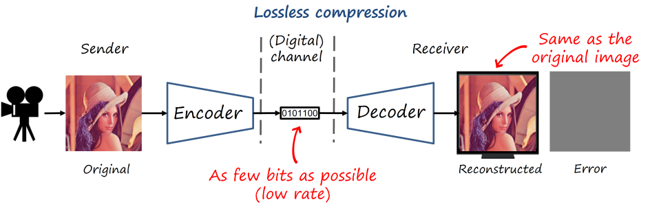
The problem of image (or video) communication deals with the transmission of a visual signal over a digital communication channel with limited capacity. The transmitting side uses an encoder to map the image to a bitstream and the receiving side uses a decoder to map it back to the image (the encoder-decoder pair is often referred to as codec).
Lossless vs lossy compression
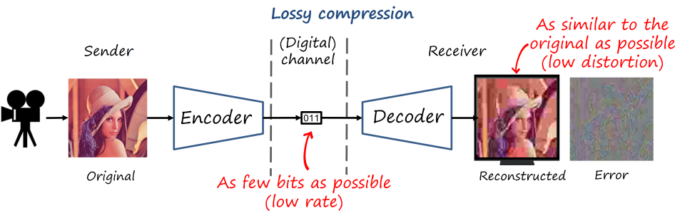
Ideally, we would like to recover the original image having transmitted as few bits as possible (that is, the lowest (bit)rate as possible). That is known as lossless compression, where we can reconstruct the original image with no error. However, visual content is still too heavy, and lossless compression still requires impractically high rates. Thus, if we need to push the compression rate much forward, the only way is by relaxing the problem so we allow some small error in the reconstructed image (i.e., low distortion), that is lossy compression. Fortunately our visual system won’t perceive many of the actual errors if we do it cleverly. Natural images also have some structural properties and statistical correlations that we can exploit. And that is the story of lossy image and video codecs: how to save bits by introducing visually imperceptible errors.
Pre/post-processing, source coding and channel coding
So far we have only described source coding, that is, mapping the source signal to a bitstream and assuming that the decoder receives exactly the same signal. In practice, the channel is not perfect and transmission may introduce errors in the bitstream. The type of coding that aims at protecting the transmitted bitstream (adding some redundancy) and allowing errors to be corrected is known as channel coding. In a general visual communications pipeline, the input signal is also pre-processed and the decoded signal is post-processed. Nevertheless, in this post we will only consider source coding.
Note that the same coding problem is not limited to transmission via a communication channel (with the bitstream received remotely). The channel itself can be a storage device where we store images or videos to decode and visualize them in the future, or distribute them in a device such as CD, DVD, or Blu-Ray.
So the lossy image coding problem involves minimizing both the distortion (i.e. de difference between the original and reconstructed images) and the rate (i.e. transmitting as few bits as possible). Additionally, there are other important practical constraints that may influence the design of the codec, such computational complexity, memory footprint and latency (e.g., mobile devices, videocalls).
In practice, specific applications impose additional constraints on the design of a codec, such as limited computational cost and low memory requirements, the ability to adjust the rate (i.e., variable rate), low latency, compatibility, etc.
Measuring rate and distortion
For the purpose of this post, we consider that the distortion D\left(x,\hat{x}\right) is the mean square error (MSE) between the original image x and the reconstructed image \hat{x}. A more practical measure is the peak signal-to-noise ratio (PSNR), which is inversely related to MSE as PSNR=10\log_{10}\left(\frac{MAX_I^2}{MSE}\right). So the lower the MSE, the higher the PSNR.
Rate in images is typically measured as bits per pixel (bpp), which is the total bits used to encode an image divided by the number of pixels in the image. As reference, an uncompressed grayscale image uses 8 bpp and a color image 24 bpp (8 bits for each color channel).
Traditional image compression: block-based (linear) transform coding
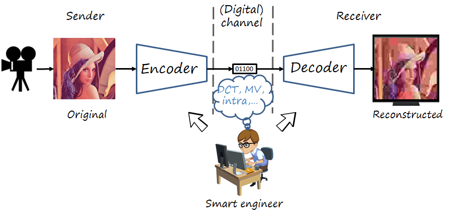
During decades the codecs were developed by expert engineers and researchers who directly design the tools and syntax and implement them in both encoder and decoder. Within this traditional approach to codec design, the most successful image and video codecs are those based on the transform coding paradigm applied on blocks (for efficiency). Examples of such approach are JPEG, MPEG-1/2/4, H.264, H.265 and VVC.
Transform coding
Although direct mapping chunks of a continuous-valued signal (we will consider images as continuous-valued) to a set of discrete symbols (i.e. vector quantization) is possible, in practice transforming it first to a more amenable feature space is preferred due to efficiency. In this paradigm, i.e., transform coding, the transformed feature is encoded using a analysis transform which largely decorrelates the dimensions in the feature space. In this way, scalar quantization can be applied (i.e., quantize each dimension independently) more effectively, and efficiently since scalar quantization is much simpler.
In traditional image coding, the transform in the feature encoder is linear and typically not learned (e.g., DCT, Fourier, wavelets), and the transform in the feature decoder is the inverse of the transform in the feature encoder. The most common transform in image coding formats is the DCT, applied in blocks of different sizes.
The output of the quantizer is a series of symbols. The next module, i.e. the entropy encoder, assigns each symbol a codeword composed of bits, according to a dictionary adapted to the probability distribution of the symbols (i.e., most common symbols will be assigned shorter codewords). Note here that accurately estimating the probability of symbols becomes an important task.
The decoder undoes the operations of the encoder, that is, the entropy decoder maps the codewords back to real values, and the feature decoder uses a synthesis transform to recover the pixel values.
Basic JPEG
Let’s take a slightly simplified version of JPEG as an example to illustrate block-based transform coding. In the following animation you can observe how the image is first partitioned into 8×8 blocks. Each block is then processed using the 2D DCT (we show 4×4 for easier visualization). We can observe how the energy is almost completely condensed into two of the coefficients. Then we apply scalar quantization, which will zero many of the coefficients, especially those related with details. The quantized coefficients are then serialized by scanning them in zig-zag order and converted to binary codewords, resulting in the bitstream. The decoder inverts the operations and recomposes the blocks, thus approximately reconstructing the image.

In the next animation we can see an example using the 2D DCT. The more coefficients are used, the lower the reconstruction error.
The DCT does a pretty good job in compacting the energy of each block in few coefficients. But, can we do better? After all the DCT is a generic transform. The Karhunen-Loeve transform (KLT) provides the optimal basis in terms of mean square error (we are essentially doing principal component analysis – PCA – ). If we vectorize each block and compute the KLT we can obtain a new set of basis and we can use it to approximate the image with even fewer coefficients. Note however that the artifacts due to block processing still remain very apparent.
In contrast to the DCT, the KLT is no longer separable and is specific to this image (so we have to save the basis in the encoder and decoder, in addition to being computationally more expensive). That is, we learned a dictionary to represent the blocks (I know, I should have used a separate training set). This shows the potential of learned codecs.
Neural image compression
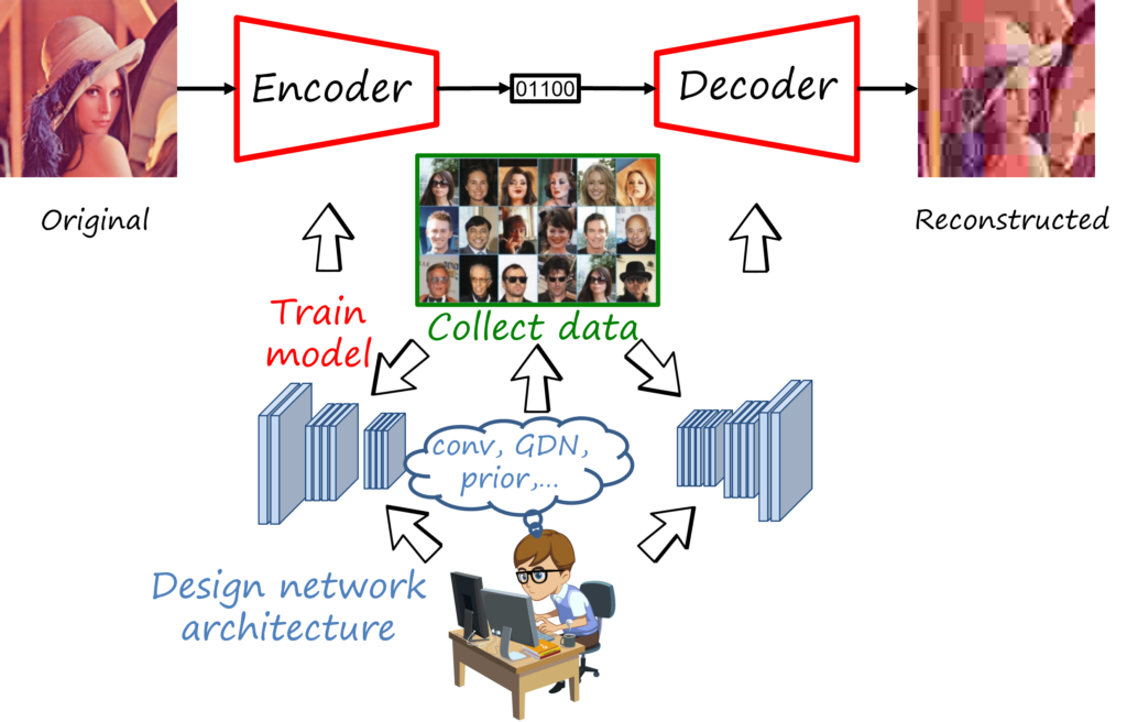
So let’s add deep learning to the mix. As everyone knows, the availability of large datasets, specialized hardware such as GPUs together with advances in architectures and training of multi-layer neural networks has radically changed the way we address problems in computer vision, natural language processing and other fields. Similarly, neural image compression adopts deep learning and its approach focused on the design of suitable network architectures and collecting suitable datasets, while the actual values of the parameters are learned through a training processs.
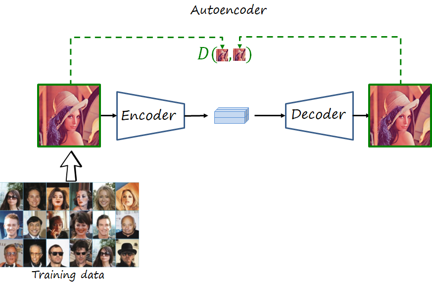
The encoder and decoder are deep neural networks trained to reconstruct the original image. If you are familiar with computer vision and deep learning, what does that remind you of? That’s right, an autoencoder, trained using a distortion metric. Its encoder maps the input image to a real-valued latent representations and its decoder tries to reconstruct the image from that latent representation, in such a way that minimizes the distortion (e.g. mean square error).
Note that we need two changes in the autoencoder to have a codec. First, the real-valued latent representation has to be serialized as a bitstream (i.e., binary stream). And second, in addition to distortion, it has to minimize the length of such bitstream (measured in bits).
Now, let’s take a step back and revisit the transform coding paradigm. We can consider the encoder and decoder of the autoencoder as deep and nonlinear transforms. We can then add the quantization and entropy coding modules, which can be parametric and even implemented deep networks themselves (we will refer to this general architecture as compressive autoencoder, as in Theis et al.). Finally, we would like to train the network (i.e., find the optimal network parameters) to explicitly minimize the rate-distortion problem (described as a weighted sum of average rate and distortion objectives evaluated over the dataset).
Wait, can we train this model?
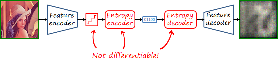
If we recall the main modules that form a codec, there are is an operation that is lossy: quantization, and two operations that are non-differentiable: quantization and entropy encoding/decoding. That is unfortunate because deep learning uses backpropagation to compute the gradients of distant layers, but backpropagation requires layers to be differentiable. Thus, we cannot backpropagate the gradients through those modules back to the feature encoder.
While the final codec will include quantization and entropy coding, during training they are replace by proxies that approximate their behavior with differentiable functions. There are different proxies for quantization, a popular one is additive uniform noise that emulates the quantization error. In the case of the entropy codec, we know that methods such as arithmetic coding can achieve lengths close to the entropy, i.e. its lower bound. Thus we simply bypass entropy coding and estimate the rate as the entropy of the quantized representation, using a learnable probability model. This probability model will then be used to construct the dictionary of the entropy codec, shared by both encoder and decoder.
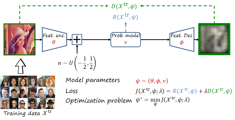
Thus, as shown in the figure, the network is composed of learnable parameters \psi=\left(\theta,\phi,\nu\right), where \theta, \phi and \nu represent the parameters of the feature encoder, feature decoder and probability model, respectively. The loss function is J\left(\mathcal{X}^{\text{tr}},\psi;\lambda\right)=R\left(\mathcal{X}^{\text{tr}},\psi\right)+\lambda D\left(\mathcal{X}^{\text{tr}},\psi\right), where rate and distortion are averaged over the training dataset \mathcal{X}^{\text{tr}} (here with a slight abuse of notation), with the two objectives weighted using the trade-off hyperparameter \lambda. The objective is to obtain the optimal parameters \psi^*.
The role of the hyperparameter \lambda: trading off rate and distortion
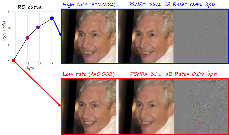
Since we have two objectives to minimize simultaneously, we have a hyperparameter \lambda that controls the relative importance of each of them. It also allows to navigate the RD curve (see following figure; bpp the lower the better, PSNR the higher the better). Focusing on distortion leads to larger bitstreams, while focusing on rate leads to higher errors in the reconstruction. Note however that \lambda is fixed and set before training, so every point in the RD curve corresponds to a different model with different parameters.
Conclusion
I hope that this post helped you understand the basic principles behind traditional and neural image compression, as well as their main differences. Traditionally, codecs have been based on block-based linear transforms and other coding tools carefully designed by engineers, while neural image compression uses deeper nonlinear transforms whose parameters are learned from data. The models are designed or learned to minimize distortion and rate, with the hyperparameter \lambda controlling the tradeoff between them.
In the second part of this post I introduce some architectural elements and entropy models designed specifically for neural image compression, and show a comparison between several compression models.
Further reading
MAE, SlimCAE and DANICE: towards practical neural image compression.
Compression for training on-board machine vision: distributed data collection and dataset restoration for autonomous vehicles.
References
J. Ballé, V. Laparra, E.P. Simoncelli, End-to-end Optimized Image Compression, ICLR 2017
L. Theis, W. Shi, A. Cunningham, F. Huszár, Lossy Image Compression with Compressive Autoencoders, ICLR 2017