Neural image codecs typically use specific elements in their architectures, such as GDN layers, hyperpriors and autoregressive context models. These elements allow exploiting contextual redundancy while obtaining accurate estimations of the probability distribution of the bits in the bitstream. Thus, the entropy codec focus only on the remaining statistical redundancy. This post briefly introduces them.
Feature autoencoder architecture
The feature encoder and feature decoder are typically based on a convolutional autoencoder architecture, where convolutions are combined with ReLU nonlinearities (see figure below, left), where the decoder mirrors the architecture of the encoder.
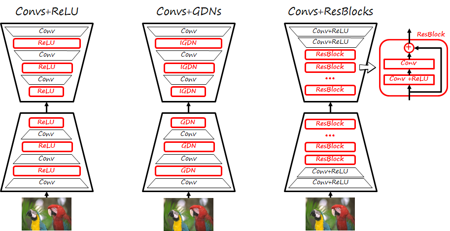
However, a more suitable architecture for image compression (see figure above, center) combines convolutional layers with a specific normalization layer called generalized divisive normalization (GDN). GDN layers are effective in shaping the distribution towards Normal ones (i.e. Gaussianization), which makes them more amenable to entropy coding. Thus, this kind of architecture requires relatively few layers, and is suitable when optimizing distortion losses. For a spatial element \left(m,n\right) and dimension i of an input tensor x the output of the GDN layer at the same element and channel is y_i\left(m,n\right)=\frac{x_i\left(m,n\right)}{\left(\beta_i+\Sigma_j\gamma_{ij}\left(x_j\left(m,n\right)\right)^2\right)^{\frac{1}{2}}} and the inverse (IGDN) is implemented as y_i\left(m,n\right)=x_i\left(m,n\right)\left(\beta_i+\Sigma_j\gamma_{ij}\left(x_j\left(m,n\right)\right)^2\right)^{\frac{1}{2}}
A third common architecture combines some convolutional layers with ReLUs and residual blocks, as those use in ResNets. The residual block has two branches, one that computes the residual via convolutional layers (typically two) and a skip connection, and the result is added. This type of architecture generally uses more layers and is often found in frameworks optimizing perceptual losses.
Entropy models
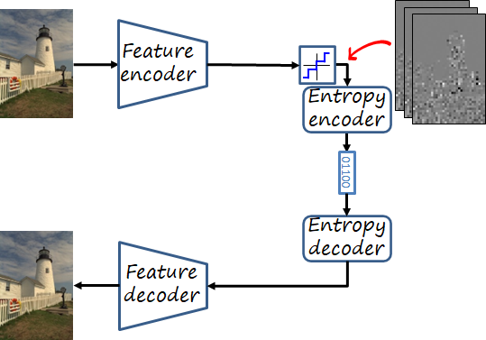
In addition to the feature encoder and decoder, a third parametric module in a neural image codec is the entropy model. A simple model can model each channel of the quantified tensor independently (known as factorized prior). However, as we can see in the figure below, there is significant correlation across spatial dimensions, as well as different scales in the values. These elements can be exploited to further reduce the rate.
Hyperprior
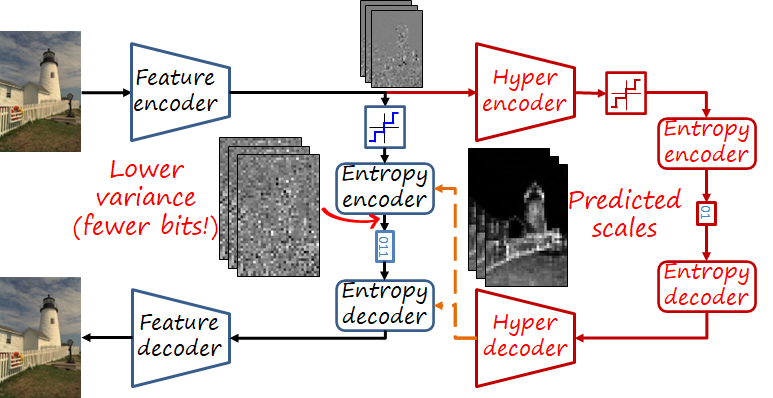
A codec with a hyperprior uses another autoencoder over the latent representation (i.e., hyperencoder and hyperdecoder). The new bottleneck representation is also quantized and entropy encoded and sent as side information (see figure below). This compact side information provides the hyperdecoder with enough information to estimate the scales of the latent representations, reducing the variance of the signal encoded by the entropy codec.
Autoregressive context model
In order to exploit spatial redundancy, some models use autoregressive models where a context composed of nearby already encoded values is used to estimate the current element (as in PixelCNN). While achieving excellent encoding performance, the sequential nature of autoregressive models makes them slow.
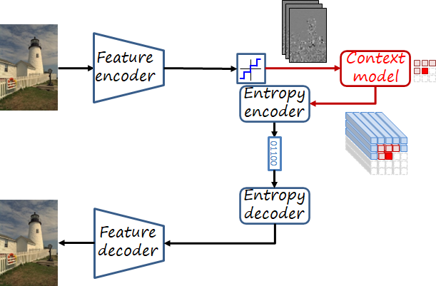
A step-by-step tour
In order to understand the encoding let’s follow the encoding and decoding processes of a neural image codec (Minnen et al. 2018) that combines both hyperprior and autoregressive context model (slides courtesy of Sudeep Katakol).

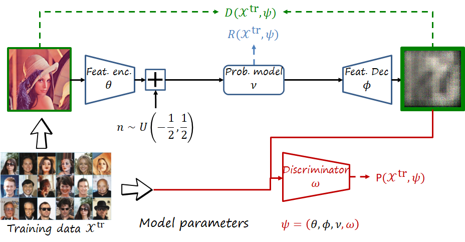
Generative image compression
Finally, a brief mention to generative image compression architectures using perceptual losses. These perceptual losses are typically adversarial losses implemented via a discriminator (as seen in the figure below). Generative frameworks optimizing perceptual losses can achieve realistic images even at very low rate (because they can hallucinate textures instead of blurring the image as happens when optimizing distortion).
Comparison
In order to illustrate the differences between the codecs, I compressed several images using Tensorflow Compression (an alternative framework is CompressAI) and several off-the-shelf models:
- bmshj2018-factorized-mse. Basic autoencoder with GDNs and a simple factorized entropy model.
- bmshj2018-hyperprior-mse. Same architecture and loss of bmshj2018-factorized-mse but with a hyperprior.
- mbt2018-mean-mse. Adds an autoregressive context model to bmshj2018-hyperprior-mse. This is the codec described step-by-step earlier.
- hific. A generative image compression framework. Uses a deeper decoder with residual blocks and minimizes adversarial loss as perceptual objective.
Select one of the following images to see a comparison between the different models.


Further reading
MAE, SlimCAE and DANICE: towards practical neural image compression.
Compression for training on-board machine vision: distributed data collection and dataset restoration for autonomous vehicles.
References
J. Ballé, V. Laparra, E.P. Simoncelli, End-to-end Optimized Image Compression, ICLR 2017
J. Ballé, V. Laparra, E.P. Simoncelli, Density Modeling of Images using a Generalized Normalization Transformation, ICLR 2016
G. Toderici, D. Vincent, N. Johnston, S.J. Hwang, D. Minnen, J. Shor, M. Covell, Full Resolution Image Compression With Recurrent Neural Networks, CVPR 2017
J. Ballé, D. Minnen, S. Singh, S.J. Hwang, N. Johnston, Variational image compression with a scale hyperprior, ICLR 2018
D. Minnen, J. Ballé, G.D. Toderici, Joint Autoregressive and Hierarchical Priors for Learned Image Compression, NeurIPS 2018
F. Mentzer, G. Toderici, M. Tschannen, E. Agustsson, High-Fidelity Generative Image Compression, NeurIPS 2020.
https://github.com/tensorflow/compression
https://interdigitalinc.github.io/CompressAI