Neural image and video codecs achieve competitive rate-distortion performance. However, they have a series of practical limitations, such as relying on heavy models, that hinder their adoption in practice. In this aspect, traditional codecs are usually designed with such practical concerns in mind. In this post I review some of our recent works focusing on these practical limitations.
If you are not familiar with neural image codecs, I suggest you first read my previous posts explaining this recent paradigm for image compression using deep neural networks (part 1, part 2). For the purpose of this post, we can consider a neural image codec as an autoencoder augmented with quantization and entropy coding and a loss J\left(\psi;\mathcal{X}^{\text{tr}},\lambda\right)=R\left(\psi;\mathcal{X}^{\text{tr}}\right)+\lambda D\left(\psi;\mathcal{X}^{\text{tr}}\right)where \psi represents the learnable network parameters, \mathcal{X}^{\text{tr}} is the training data and \lambda is the rate-distortion (RD) tradeoff. The loss is minimized for \psi, given \mathcal{X}^{\text{tr}} and \lambda.
Practical issues with neural image codecs
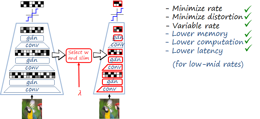
Most research in neural image and video compression has focused on optimizing rate and distortion as unique objectives. However, real applications usually require considering other practical requirements which are often overlooked in the neural image/video codec literature, such as variable rate, computation and memory costs, latency and codec adaptation and compatibility. In this post I review three of our recent works in that direction: modulated autoencoders (MAE), slimmable compressive autoencoders (SlimCAE) and domain adaptive neural compression (DANICE). The following figure enumerate the limitations of a typical neural image codec, and which practical aspects are addressed in each of the papers.
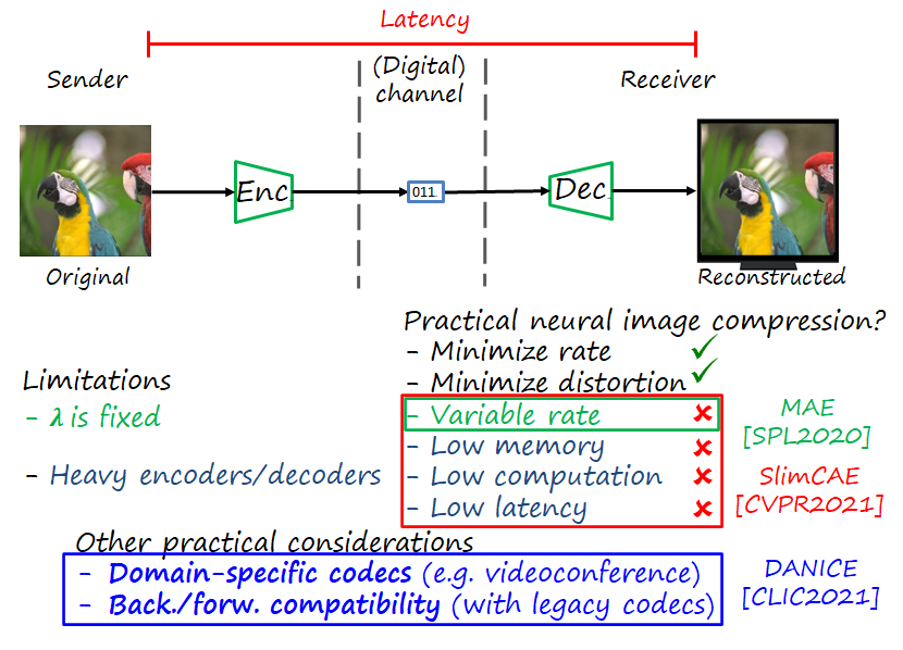
As you can see, the main limitations arise from the large size of neural image encoders and decoders, and the fact that they are optimize to a particular RD tradeoff.
MAE: variable rate via feature modulation
Most codecs simply minimize a weighted sum of rate and distortion R+\lambda D, where the tradeoff is controlled by the hyperparameter \lambda. Thus, by construction, the model is only optimal for that specific tradeoff \lambda it was trained for. This is an important limitation in practice, since providing variable rate (i.e., the functionality to vary the rate-distortion tradeoff on demand) in an optimal way requires training multiple models, as many as desired rate-distortion operational points. The obvious drawback is that all those models need to be stored in the device, with a significant increase in storage requirements, and the potential cost of switching from one model to another when necessary. These limitations are particularly important in video compression where rate control is a more crucial requirement.
An early neural image codec providing variable rate capability is the compressive autoencoder (CAE) of Theis et al. Their approach (here referred to as bottleneck scaling) is a direct adaptation of the quantization parameters and matrices used in traditional codecs such as JPEG, i.e., each channel of the latent representation at the bottleneck is scaled by a constant factor before quantization, and descaled by the same factor in the decoder. The scaling factors are different for different \lambdas, and stored in a table known by both encoder and decoder.
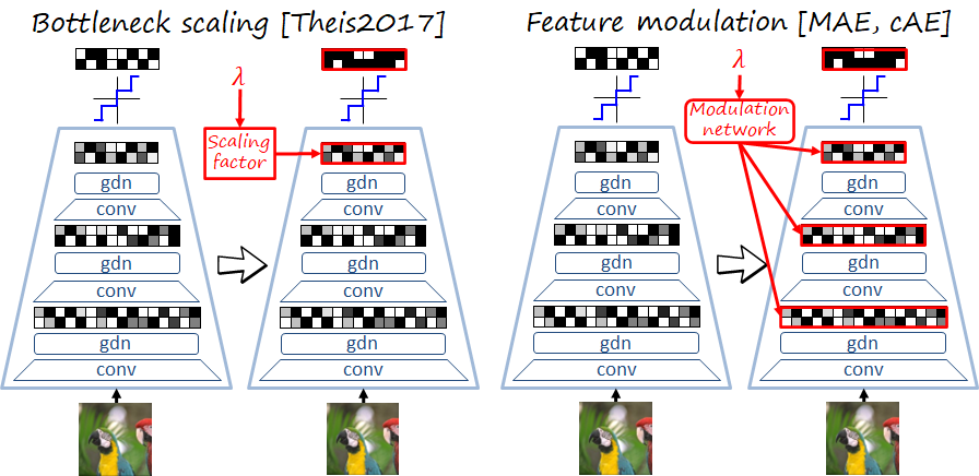
While scaling the bottleneck representation can effectively control the rate, we observed an RD performance drop with respect to training independent models, especially at low rates. In order to increase the flexibility of the model to adapt to different RD tradeoffs, we propose a modulated autoencoder (MAE) where not only the bottleneck but also intermediate representations are modulated. Instead of using scale factors, the relation of the modulation parameters with \lambda is learned by a a simple modulation network in encoder (demodulation network in decoder). The new training loss is J\left(\psi,\vartheta,\varphi;\mathcal{X}^{\text{tr}},\Lambda\right)=\sum_{\lambda \in \Lambda}\left[R\left(\psi,\vartheta,\varphi;\mathcal{X}^{\text{tr}},\lambda\right)+\lambda D\left(\psi,\vartheta,\varphi;\mathcal{X}^{\text{tr}},\lambda\right)\right]where \vartheta and \varphi represent the parameters of the modulation and demodulation networks, respectively, and \Lambda=\left\{\lambda_1,\ldots,\lambda_M\right\} is the fixed set of target RD tradeoffs. The loss is jointly minimized for \psi, \varphi and \vartheta. This approach allows us to provide variable rate with one model with almost no penalty in RD performance. Note that Choi et al. concurrently proposed a similar method referred to as conditional autoencoders -cAE-.
SlimCAE: slimming the codec to reduce computation and memory
The previous variable rate models (CAE+scaling, MAE, cAE) can reduce the number of models to one, thus saving significant memory. However the model still remains heavy and computationally expensive. Now we focus on reducing the size of the model itself to achieve lightweight models that require less memory and lower computation, also resulting in lower latency.
A key observation: rate-distortion and model capacity
We performed the following experiment: we train many compressive autoencoders with different capacities (by varying the width of convolutional layers, i.e. the number of filters in the layer) and different RD tradeoffs, so we can plot the RD curve for different capacities. The figure below illustrates the resulting curves.
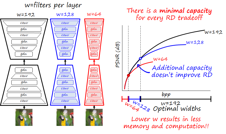
We observe that below a certain rate the curves of certain width or higher overlap. That means that additional capacity is of no use below that rate. We observe that this behavior is also consistent for different curves with different widths. This suggest that there is a minimum capacity (parametrized by width w_i in our case) for every RD tradeoff \lambda_i.
Intuitively this makes sense: with fewer bits in the bitstream we can only signal few combinations of filters. Since we are using MSE as distortion metric, we cannot signal many combinations, and approximating lower frequencies is a priority since it reduces MSE more significantly than high-frequency details. Therefore, decoder filters that reconstruct details will be rarely used (if ever) at low rates, and similarly, the encoder won’t signal that information, so encoder filters that analyze and encode details are also likely not necessary.
This observation has already a practical application: we can reduce the memory used by independent models by designing them with the optimal width for a given RD tradeoff. Now the question is: can we apply this finding to variable rate models? In the case of the previously described ones the answer is no, since they still require using the maximum capacity in order to encoded the highest rate.
Slimmable compressive autoencoders
Slimmable networks organize the filters in a way that they can reduce the capacity of the model (via adjusting the width) still and operate and designing an slimmable codec. We apply this design principle to our CAE, hence named Slimmable CAE (SlimCAE). Here we are adding an additional constraint: a submodel i contains and shares the weights of submodels i'<i, with widths w_i'<w_i. As we saw before, we can still achieve optimal RD performance for a certain set of tradeoffs \Lambda=\left\{\lambda_1,\ldots,\lambda_M\right\}, even with this additional restriction. Once the architectures of the subCAEs are organized in this way, we can by slimming the CAE, i.e., selecting the subCAE of width w_i corresponding to the RD tradeoff \lambda_i, and discarding the rest of parameters.
Architecture: slimmable convs and slimmable GDNs
Our architecture is based on that of Balle et al., which combines convolutional layers and generalized divisive normalization (GDN) layers. Thus, an SlimCAE has to implement slimmable versions of these two layers, as shown in the figure below. The slimmable convolutions are straightforward and used in previous works using slimmable networks.
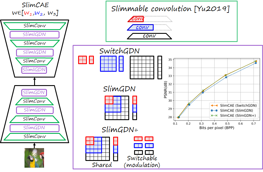
GDN layers are popular in neural image compression. We develop three slimmable variants of this type of layer:
- SwitchGDN. This variant is not slimmable (while the convolutions still are), it simply has different sets of parameters for different i. The drawback is that increases the number of parameters.
- SlimGDN. This variant is slimmable, since parameters of each subGDN are shared with the higher subGDNs. The drawback is that we observed a drop in RD performance.
- SlimGDN++. This variant contains a SlimGDN and a set of switchable feature modulation parameters (scale and bias per channel). This variant achieves the optimal performance of SwitchGDN at a negligible increase in number of parameters.
How to train the model? Do we even know the optimal \lambda for a given capacity?
Ok, we have a CAE architecture (and its subCAEs) and a adaptation mechanism. Our objective is to minimize the following loss J\left(\psi,\Lambda;\mathcal{X}^{\text{tr}}\right)=\sum_{i=1}^K\left[R\left(\psi^{\left(k\right)};\mathcal{X}^{\text{tr}}\right)+\lambda_k D\left(\psi^{\left(k\right)};\mathcal{X}^{\text{tr}}\right)\right]where \psi^{\left(1\right)}\subset\cdots\subset\psi^{\left(K\right)}=\psi.
Now we can define a set of widths and the corresponding subCAEs. But, how do we know the corresponding optimal values of \lambda. One possible way is to precompute the RD curves for the corresponding widths by training multiple independent models at different \lambdas and find the critical points where curves diverge. The problem with this method is that requires training too many models.

In order to avoid the previous cost, we propose \lambda-scheduling, an alternating optimization approach that can learn \psi and \Lambda simultaneously. We start with a naive solution where \lambda_1=\cdots=\lambda_K (admittedly, not the best initialization), and then alternate between training the CAE and updating \Lambda following a schedule, in a way that the curve will progressively approximate the convex hull of all RD curves, i.e., our target RD curve. In this way we only train one model, yet still achieving optimal results.

Experimental comparison
The next figures shows some experimental results comparing MAE, SlimCAE and some baselines (independent models, CAE+scaling, cAE). In general, the upper bound is given by independent models. Here we use the observation described before and only use optimal models with the minimal capacity. Note how for low rates the memory footprint, computational cost and latency can be reduced dramatically. But we need to save all the models and switch between them.
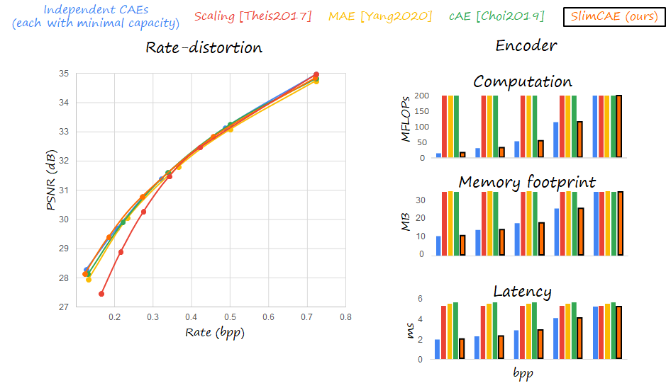
MAE and cAE can provide essentially the same RD performance as independent models, thanks to the modulation mechanism. In contrast, only scaling the bottleneck representation is not enough, since it leads to drops in performance. The slimming mechanism in SlimCAE is equally effective.
The main advantage of SlimCAE over MAE and cAE is that it only requires a fraction of the parameters for low and mid rates, thus reducing significantly the computation, memory footprint and latency.
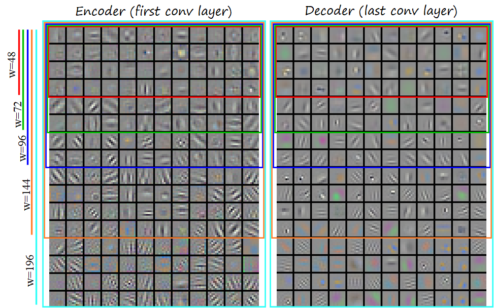
Some insights from slimmable convolutions
Visualizing the convolutions closest to the pixels, that is, the first convolution of the encoder and the last convolution of the decoder illustrate how the filters become organized in a clear pattern (see figure below). Low frequency patterns tend to emerge in smaller subCAEs, while higher frequencies progressively appear as the width increases.
DANICE: neural image compression meets domain adaptation and continual learning
The nature of neural image codecs as deep learned models opens doors to new functionalities and connections machine learning fields. In this work we focus on providing a new functionality of codec adaptation to custom user domains, which is connected to the problems of transfer learning and domain adaptation in machine learning. Then we extend the work towards keeping it functionality in the source domain, which in turn is connected to the problem of continual learning, and to the traditional concept in image coding of backward compatibility.
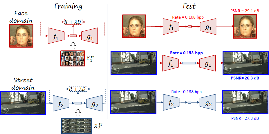
An obvious characteristic of neural image codecs is that they are optimal for the domain of the data they were trained with. For example, if a codec is trained with face images, they will have good RD performance when encoding face images. But their performance will be suboptimal when encoding street images, at least compared with a codec trained with street images (i.e. higher rate and higher distortion).
Codec for custom domains
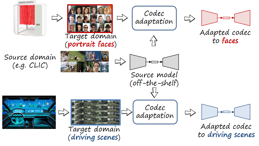
Since neural image codecs can learn from data, in principle, neural image codecs could learn from the photos taken by a user. For example, an off-the-shelf codec deployed in a photo booth or a studio specialized in portraits could learn to better compress face images directly from the photos taken by the user. Thus, we introduce the idea of codec adaptation, where an off-the-shelf codec trained on a generic dataset (e.g. CLIC dataset) can be optimized by the user to her custom domain. Note that the user data can be limited, so in order to have competitive RD performance in the target domain we benefit from the pretrained model trained in a generic source domain.
Codec compatibility as a continual learning problem
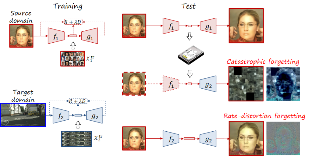
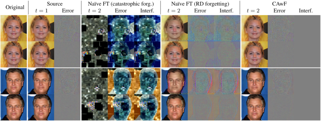
Now let us consider the following situation: at time 1 the user has a codec trained in a source domain, and then at time 2 adapts it to a target domain (e.g., from CLIC to faces, or from faces to street scenes as in the following figure). In codec adaptation we only care about the performance in time 2, but what if we want to decode compressed images encoded at time 1? Or ocassionally take and encode photos of the source domain? In both scenarios the new codec is suboptimal, leading to what in machine learning is know as forgetting. We distinguish between two types of forgetting, corresponding to the previous two cases:
- Catastrophic forgetting. When trying to decode with a time 2 decoder a bitstream encoded with a time 1 encoder, the mismatch between both leads to a truly catastrophic result, because the resulting image is pretty much a random image that doesn’t resemble the input image. This scenario is analogous to the incompatibility between two traditional codecs (or profiles) that don’t share the same syntax, and therefore can’t communicate. In the learned codec the syntax corresponds to the quantized latent space, while in the traditional case is handcrafted.
- Rate-distortion forgetting. When using a time 2 encoder and decoder to process images of the source domain, the result is not catastrophic, and we can obtain the input image. However, the bitstream is likely to be larger and the reconstructed image will likely exhibit degradation and artifacts. Due to adaptation, the codec has forgotten its original rate-distortion capability in the source domain.
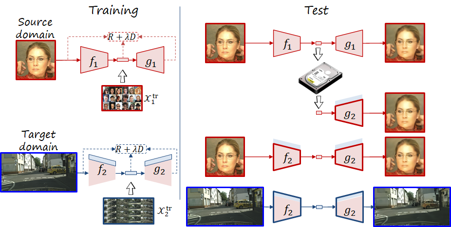
The phenomenon of forgetting has been studied in the field of continual learning. In order to prevent the forgetting issues described above, we propose a codec adaptation method (i.e., codec adaptation without forgetting or CAwF) based on parameter-isolation. During adaptation, the source codec (i.e., time 1) remains frozen, and the target codec (i.e., time 2) is composed by the frozen parameters and a small subset of new trainable parameters. In this way, we have both the source codec and target codecs embedded in the same model, and can be retrieved as necessary (signalling the version of the codec requires only one additional bit). This approach can keep bitstreams and decoders compatible over time, while also keeping the source performance, at the cost of a number of additional parameters.
The following figure shows some examples of the different cases at low and high rates and the resulting errors and artifacts.
References
F. Yang, L. Herranz, J. van de Weijer, J.A. Iglesias Guitián, A. López, M. Mozerov, “Variable Rate Deep Image Compression with Modulated Autoencoders”, IEEE Signal Processing Letters, Jan. 2020 [arxiv] [link].
F. Yang, L. Herranz, Y. Cheng, M. Mozerov, “Slimmable compressive autoencoders for practical neural image compression”, Proc. International Conference on Computer Vision and Pattern Recognition (CVPR21), June 2021 [arxiv] [slides] [video].
S. Katakol, L. Herranz, F. Yang, M. Mrak, “DANICE: Domain adaptation without forgetting in neural image compression”, CVPR Workshop and Challenge on Learned Image Compression (CLIC 2021), June 2021 [arxiv] [slides] [video].
J. Ballé, V. Laparra, E.P. Simoncelli, End-to-end Optimized Image Compression, ICLR 2017
L. Theis, W. Shi, A. Cunningham, F. Huszár, Lossy Image Compression with Compressive Autoencoders, ICLR 2017
Y. Choi, M. El-Khamy, J. Lee, Variable Rate Deep Image Compression With a Conditional Autoencoder, ICCV 2019
J. Yu, L. Yang, N. Xu, J. Yang, T. Huang, Slimmable Neural Networks, ICLR 2019