
Depth sensors capture information that complements conventional RGB data. How to combine them in an effective multimodal representation is still actively studied, and depends on different factors. Here I will focus on scenes and discuss several approaches to RGB-D scene recognition, although the discussion can probably apply also to other tasks, such as object detection or segmentation.
There are several factors that should be considered while learning RGB-D features:
- Amount of modality-specific data available.
- Intrinsic complexity of each modality.
- Practical limitations of modality-specific sensors.
Visual recognition on RGB-D images
Let us start with images first. In general, the RGB-D recognition pipeline includes two streams (one for RGB and another for depth). The inputs are RGB-D image pairs that are fed to each stream, and then the two modality-specific features are combined at some point in the processing. The next figure shows the usual pipeline:
RGB representations: Places-CNN
The RGB modality has large databases (e.g. Places, LSUN), which enable training deep networks that extract good RGB features. In particular, Places has millions of images and hundreds of categories. The RGB branch is obtained by fine-tuning a Places-CNN.
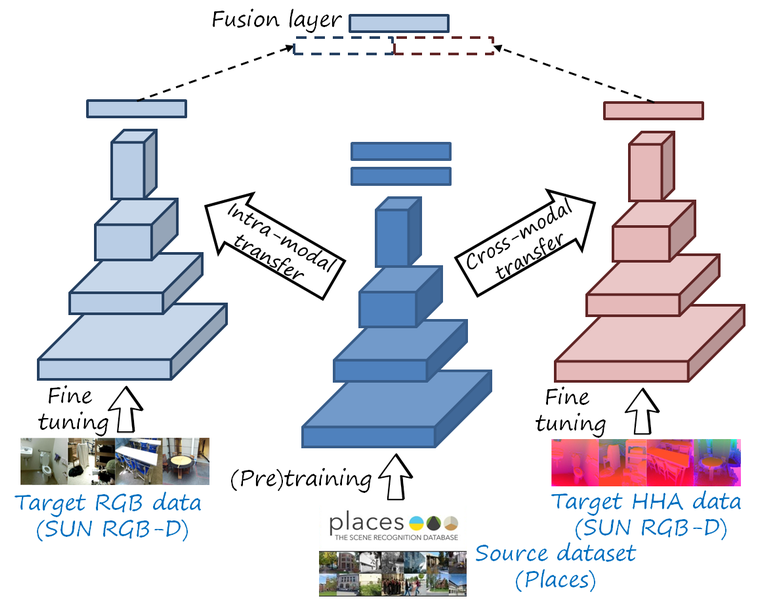
Depth representations: HHA encoding and cross-modal transfer
However, there is no equivalent large database for depth data of real scenes, since collecting depth data is more expensive (in contrast to RGB, depth images from real scenes cannot be crawled from the web). A common approach is using cross-modal transfer from a deep RGB network, trained with a large RGB dataset. Gupta et al. proposed HHA, a geocentric embedding which converts a one channel-depth image into a three-channel image: horizontal disparity, height above ground and angle with gravity.

In contrast to the original depth images, HHA images have the same number of channels as RGB, and note that many objects are recognizable since many patterns are similar to those in RGB, such as borders, shapes and gradients. So perhaps RGB networks, fine tuned with the limited HHA data could be effectively adapted to this modality. In fact, the authors hypothesize that there is “enough common structure between our HHA geocentric images and RGB images that a network designed for RGB images can also learn a suitable representation for HHA images”. And indeed there is, and they show in their experiments that initializing the networks with a network trained ImageNet obtained better results that with random initialization (note the results are for object detection in the NYU2 dataset).
The larger SUN RGB-D dataset was proposed in CVPR 2015, with more images than NYU2 (5285 vs 795 images), and the authors show that having more images for fine tuning improves performance, as expected. But they still rely on fine tuning a Places-CNN. This type of cross-modal transfer (i.e. from RGB to depth) to learn depth representations with deep networks has been widely adopted in the RGB-D community.
Correlation and redundacy at high-level features
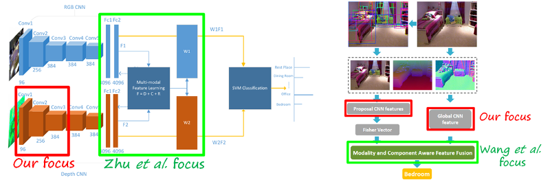
Many papers about RGB-D recognition have adopted this architecture with two modality-specific sub-networks, both initialized with a network trained on Places, a.k.a. Places-CNN (in the case of scene recognition; usually ImageNet in other tasks). The features from both streams are usually combined simply by concatenating them, and further processed jointly. Since there is correlation and redundancy between the features extracted from both modalities, many papers address the problem of how to exploit them to obtain more compact and discriminative multimodal features in order to increase the recognition accuracy. For instance, the following figure shows two works from CVPR 2016 (Zhu et al. and Wang et al.). Both focus on combining both modalities in a more discriminative and compact way to improve the accuracy.
Addressing the correlation and redundancy between modality-specific high-level features will lead to some important gains in accuracy. However, this is due to the fact that each stream is based on Places-CNNs, which results in features with high redundancy and correlation in the first place. But perhaps avoiding correlation and redundancy in the first place may be better. This is precisely the focus in our work.
Taking a step back. Is transferring from RGB to depth a good idea?
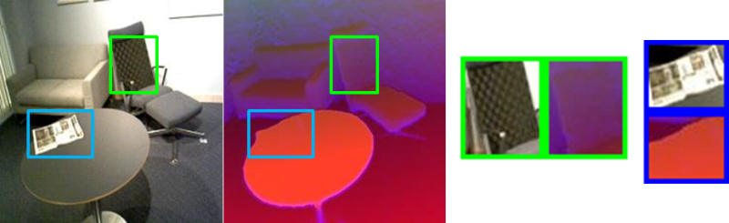
Let us take a closer look to the previous example of an RGB-D image pair (in fact RGB and HHA images). We can observe that shapes and borders appear in both images making objects recognizable. However, there are also features that appear differently in each modality. For instance, textured regions with high frequency components do not appear in the HHA image (e.g. newspaper, back of the chair). Sometimes, similar patterns appear but with different meanings in each modality, such as smooth gradients (e.g. indicate changes in illumination in RGB while indicate change in distance in HHA).
So there are some typical patterns in RGB images that also appear in HHA images (some of them with different interpretation) and some that do not appear. This leads to the question: does a (fine tuned) Places-CNN (trained with RGB data) actually extract good features for depth modality? We performed the following experiment: took a Places-CNN (AlexNet architecture, not fine tuned) and observed the activations in the conv1 layer, measuring the average non-zero activations and the mean activation of the filters (see next figures).
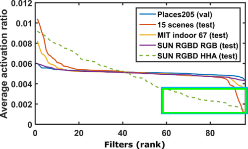
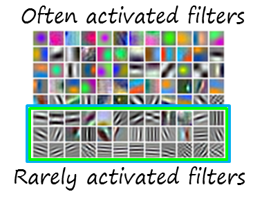
We observe that when tested on other RGB scene images (i.e. intra-modal transfer) the results are fairly flat curves indicating a well balanced layer where most filters are used with similar frequency, even on target RGB sets (including RGB images of SUN RGB-D). In contrast, when tested on the HHA images from SUN RGB-D (i.e. cross-modal transfer), the curve is much more skewed, indicating an important imbalance suggesting some filters are used often while others are rarely used. This leads to redundant and noisy depth representations. We can also observe that the less frequently used filters are related with texture and high frequency components, while the most frequently used are related with gradients and contrast between colors (although in HHA encoding have a geometrical meaning rather than in terms of color).
So it seems that cross-modal transfer from Places-CNN is not optimal, unless you prefer solving the problem of noise and redundancy at later stages.
Learning good depth representations from scratch
We believe that a better strategy is to learn compact and complementary depth features from the very beginning, so in our recent work (presented at AAAI 2017) we focus on early processing stages of depth data (i.e. bottom layers of the HHA sub-network) rather than addressing the problem later stages. In that way we avoid redundancy by learning modality-specific low-level features, which can also be more complementary. In particular, we observed that in our cross-modal adaptation case, fine tuning bottom layers is more critical than higher layers (in contrast to conventional fine tuning for intra-modal adaptation, which fine tunes upper layers).
The main challenge is to learn good and discriminative features with such limited data (only around 5000 thousand images). Two remarks: (1) HHA is much less complex than RGB, so a simpler model may suffice to capture depth-specific discriminative patterns, and (2) training a simpler model with fewer parameters requires a smaller amount of samples. The question is: would that model be powerful enough to compete with fine tuned Places-CNN (trained with millions of images)? In many previous work it was assumed that it would not.
In this work we propose to use a simpler network, since AlexNet is too complex for HHA data. Our network (referred to as Depth-CNN) has four convolutional and two fully connected layers, with fewer filters. However, the amount of data is still limited to train the full network. We propose to train the network in two steps: (1) pre-train the four convolutional layers with patches in a weakly supervised manner, and (2) train the full network with full images.
In the first step, we reduce the receptive field by working on patches in such a way that the output of the fourth convolutional layer is just a vector (being effectively a fully connected layer). In this way the network has fewer parameters while then number of input samples increases since a single image has multiple patches. Since we do not have suitable labels for the patches (which would be at the scale of objects), we use the global scene category. Hence, the features are learned in a weakly supervised manner.
In the second step, the fully connected layer is reshaped into a convolutional network, and a spatial pyramid and two more fully connected layers are added. Now the receptive field corresponds to full images, which are used to train the full network. The weakly supervised model provides a good initial solution, so the second step can focus on the latest stages.

Modality-specific features are more complementary
The following shows the results of our experiments on SUN RGB-D (using AlexNet architectures for Places-CNN).
| Method | CNN models | Accuracy (%) | Gain over best single modality (%) | ||||
| RGB | HHA | RGB | HHA | RGB-D | |||
| Baseline | Concat. | PL | PL | 35.4 | 30.9 | 39.1 | +3.7 |
| Concat. | FT-PL | FT-PL | 41.5 | 37.5 | 45.4 | +3.9 | |
| Concat. (wSVM) | FT-PL | FT-PL | 42.7 | 38.7 | 46.9 | +4.2 | |
| Proposed | Concat. | FT-PL | FT-WSP-ALEX | 41.5 | 37.5 | 48.5 | +7.0 |
| RGB-D-CNN | FT-PL | D-CNN | 41.5 | 41.2 | 50.9 | +9.4 | |
| RGB-D-CNN (wSVM) | FT-PL | D-CNN | 42.7 | 42.4 | 52.4 | +9.7 | |
| Other works | Zhu et al. CVPR 2016 | FT-PL | FT-PL | 37.0 | – | 41.5 | +4.1 |
| Wang et al. CVPR 2016 | FT-PL + R-CNN | FT-PL + R-CNN | 40.4 | 36.3 | 48.1 | +7.7 | |
| Song et al. IJCAI 2017 | FT-PL | FT-PL + ALEX | 41.5 | 40.1 | 52.3 | +11.2 | |
Results on SUN RGB-D. FT: fine tuned, PL: Places-CNN, WSP: weakly supervised with patches, ALEX: AlexNet (from scratch), wSVM: weighted SVM.
The depth features learned with the proposed method are competitive with fine tuned Places-CNN (42.4% with D-CNN vs 42.7% FT-PL, both with wSVM), but without requiring access to a large RGB dataset. More importantly, these features are truly depth-specific, so there are more complementary than those from fine tuned Places-CNNs, so the gain when combined in the RGB-D framework is higher (+9.7% vs +4.2%).
Note that our method is much simpler than the other related methods. Zhu et al. uses two branches and a more complex discriminative fusion layer to reduce covariance at high-levels. Want et al. uses a much more complex architecture integrating three modalities (RGB, HHA and surface normals) and two additional streams for each modality (global and local using R-CNN and Fisher vectors to pool them). Note that we have better accuracy and higher gain with a much simpler and efficient approach thanks to learning truly depth-specific features from the very bottom. Our related work Song et al. also has a three branch architecture and more complex fusion method based on searching of good combinations of layers. The gain is higher, but at the cost of a more complex architecture and design.
Scene recognition on RGB-D videos
Another difference between RGB and depth modalities is that the depth sensor has a much more limited distance range, not capturing distant objects, while the RGB one can. You can see the difference in the following example.
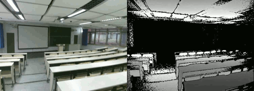
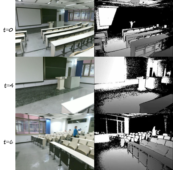
Note how the RGB sensor can capture the black board and windows at the right side while the depth sensor is not able to (at t=0). As the camera moves across the scene, new information appears in both RGB and depth modalities, especially in the latter due to the limited range. That motivates the extension of our approach to RGB-D videos (accepted by IEEE Trans. on Image Processing). In this case the key is to accummulate the depth information, so we evaluated different ways, including average pooling and recurrent neural networks (long short-term memory -LSTM- in particular).
In order to evaluate this scenario, we collected a dataset (ISIA RGB-D video database) to evaluate scene recognition in wide scenes. The following figure summarizes the findings.
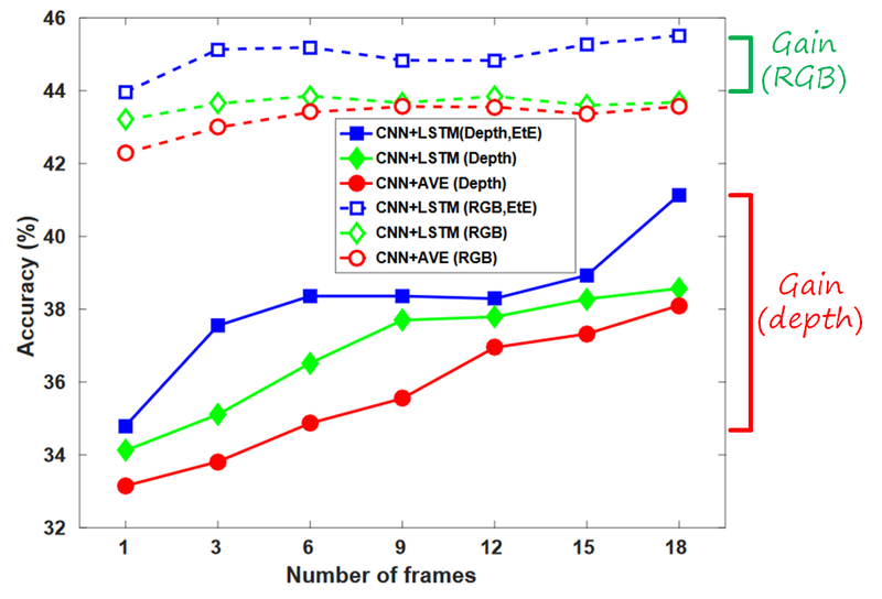
We compared three extensions of our previous method to sequences: average pooling, LSTM and LSTM trained end-to-end. While processing more frames helps to improve the representation, the gain is more significant in depth than in RGB (around 6% vs around 1.5%). End-to-end LSTM also delivers the higher gains in both cases.
In conclusion, we analyzed different ways to extract depth features for scene recognition with convolutional neural networks. We showed that the widely used cross-modal transfer and fine tuning (Places-CNN to depth) is not necessarily the best solution, since low-level layers are still too specific to RGB patterns. Even with limited data, it is possible to learn from scratch models that extract truly depth-specific features, which are more complementary to RGB ones, and yield higher gains when combined. Similarly, higher gains in RGB-D videos can be obtain when accumulating depth information from several frames, alleviating the limitation of the limited range in depth sensors.
References
X. Song, S. Jiang, L. Herranz, C. Chen, “Learning Effective RGB-D Representations for Scene Recognition” , IEEE Transactions on Image Processing, vol. 28, no. 2, pp. 980-993, Feb. 2019 [arxiv] [link]