Can we perform unsupervised domain adaptation without accessing source data? Recent works show that it is not only possible but also very effective. In this post I review our recent works (ICCV 2021, NeurIPS 2021, CVIU 2023 and TPAMI 2023), where we tackle this challenging setting known as source-free unsupervised domain adaptation (SFUDA), and propose new extended settings (namely online, generalized and continual SFUDA).
Unsupervised domain adaptation and the source-free constraint
A fundamental advantage of deep learning is that the knowledge learned by the models from a particular data-rich source dataset can be effectively transferred, reused and adapted to many related target tasks and domains where data is more limited, and often not annotated. This broad field is known as transfer learning. The particular case where the task does not change (e.g. classifying into the same categories) but the input distribution does (e.g. the source domain consists of synthetic images and the target domain of natural images) is known as domain adaptation (DA). The general supervised case assumes that images and labels (we will focus here on classification) are available in both source and target domains.
However, not only collecting data is expensive and time consuming, but so it is labeling the data. Thus, unsupervised domain adaptation (UDA), where target data is not annotated, is perhaps the setting of most practical interest. For example, the following figure illustrates a case where a source dataset with abundant annotated data is leveraged to tackle a target dataset with images of the same classes, but with more complex poses and backgrounds, fewer samples and lacking labels.
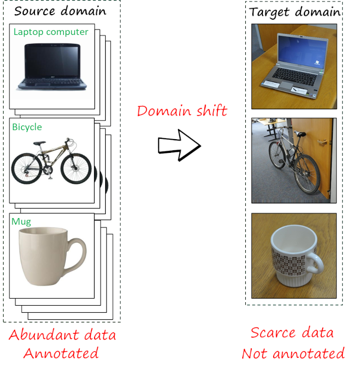
Most UDA approaches assume that both source and target data are available during the adaptation process. However, there are numerous cases in which source data is not accessible. For example, source data often contain private data, preventing its sharing. Similarly, storing source data may be not possible in resource-limited scenarios, such as adaptation in mobile devices. This new constraint motivates the increasing interest in source-free unsupervised domain adaptation (SFUDA), which is the focus of this post.
Different scenarios and applications may further lead to additional constraints and requirements. I describe some in the second part of this post. For more details on SFUDA, I refer the reader to a recent survey, while here I will focus more specifically on our approaches.
Methods
Preliminaries and notation
Let’s first introduce some notation. We focus on C-way classification tasks. We consider source domain data \mathcal{D}_s=\left\{ \left ( \mathbf{x}_s^i,y_s^i \right )\right\}_{i=1}^{n_s} where each sample \mathbf{x}_s^i has a corresponding label \mathbf{x}_s^i. The target domain data \mathcal{D}_t=\left\{ \left ( \mathbf{x}_t^j\right )\right\}_{j=1}^{n_t} is unlabeled. Both source and target models are implemented as deep neural networks p\left(\mathbf{x}\right)=\delta\left(g\left(\mathbf{z}\right)\right)=\delta\left(g\left(f\left(\mathbf{x}\right)\right)\right), where f, g, \delta and p denote the feature extractor, classifier, softmax and output probabilities, respectively. We also denote the intermediate feature obtained by the feature extractor as \mathbf{z}=f\left(\mathbf{x}\right). In most cases we will operate with \mathbf{z} and p, often omitting the explicit dependency on \mathbf{x}, for the sake of readability. Under SFUDA, \mathcal{D}_s is only available during the (pre)training of the source model. The source data then becames unavailable, but the source model (i.e. source feature extractor f_s and source classifier g_s) remain available.
SHOT: a popular method
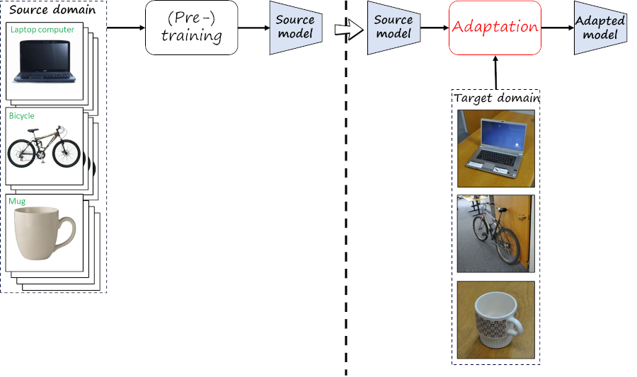
Before introducing our approaches, I will briefly review Source HypOthesis Transfer (SHOT), which is a popular method and which we use as baseline. SHOT is based on the idea of hypothesis transfer, where the hypothesis is represented by the source classifier which remains fixed during the adaptation process. In this way, the objective is to align the target features obtained by the adapted feature extractor to the source classifier (i.e. hypothesis), as illustrated in the following figure.
The source model is first learned using supervised learning via minimizing the cross-entropy loss \mathcal{L}\left(f_s,g_s;\mathcal{D}_s\right)=-\frac{1}{n_s}\sum_{i=1}^{n_s}\sum_{c=1}^C \mathbf{I}_{\left[c=y_s^i\right]}\log \delta_c\left(g_s\left(f_s\left(x\right)\right)\right)=-\frac{1}{n_s}\sum_{i=1}^{n_s}\sum_{c=1}^C \mathbf{I}_{\left[c=y_s^i\right]}\log p_c\left(x\right) where the indicator function \mathbf{I}_{\left[u\right]} is 1 when u is true, 0 otherwise, and \delta_c is the c-th dimension of the softmax vector.
Adaptation begins by transferring the feature extractor f_t=f_s and the classifer g_t=g_s. While f_t is updated, the classifier g_t (i.e. hypothesis) remains frozen. The source-free unsupervised adaptation process minimizes a combination of information maximization loss and a self-supervised pseudo-labeling loss. In particular, the total loss is
\mathcal{L}\left(f_t;\mathcal{D}_t\right)=\underbrace{\underbrace{-\frac{1}{n_t}\sum_{i=1}^{n_t}\sum_{c=1}^C \delta_c\left(g_s\left(f_s\left(x\right)\right)\right) \log \delta_c\left(g_t\left(f_t\left(x\right)\right)\right)}_\text{Entropy}+\underbrace{\sum_{c=1}^C \hat{p}_c \log \hat{p}_c}_\text{Diversity}}_\text{Information maximization}-\beta\underbrace{\frac{1}{n_s}\sum_{i=1}^{n_s}\sum_{c=1}^C \mathbf{I}_{\left[c=\hat{y}_t^i\right]}\log \delta_c\left(g_s\left(f_s\left(x\right)\right)\right)}_\text{Pseudo-labels} is the pseudo-label for \mathbf{x}_i. Pseudo-labels are obtained by computing class centroids and then labels are estimated using a nearest centroid classifier. The information maximization combines entropy minimization and a diversity loss. Note that the diversity term aligns the average predicted probability with the uniform distribution, i.e. \sum_{c=1}^C \hat{p}_c \log \hat{p}_c=D_\text{KL}\left(\hat{p}\lVert \frac{1}{C}\mathbf{1}_C\right)-\log C, where the average predicted probability is estimated as \hat{p}=\frac{1}{n_t}\sum_{i=1}^{n_t} p_c\left(\mathbf{x}_i\right) and \mathbf{1}_C is a vector with C ones.
BAIT (CVIU 2023)
Our first work is similar to SHOT in that transfers and keeps fixed the source hypothesis (i.e. source classifier). However, it differs in the adaptation method, which in our case uses a auxiliary classifier (i.e. bait classifier) that acts as a bait to attract uncertain data towards the certain data. The entropy of the output predictions serve as mechanism to split target features into certain (i.e. low entropy) and uncertain (i.e. high entropy).
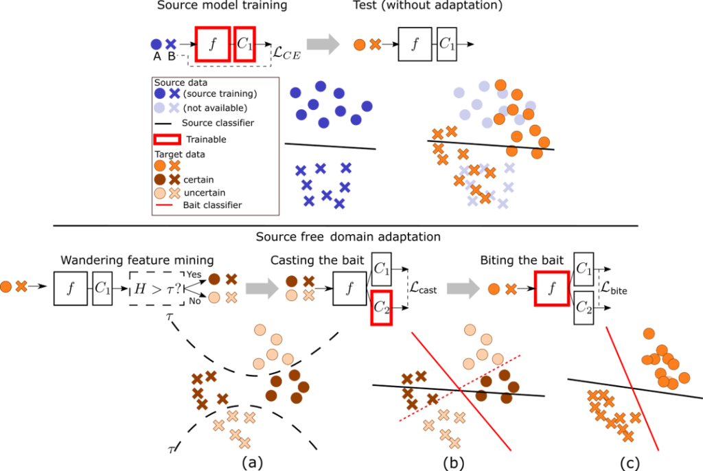
The adaptation algorithm iterates between three steps:
- Feature mining. The target data is separated into two subsets: certain features \mathcal{C}=\left\{\mathbf{x}\vert \mathbf{x}\in \mathcal{D}_t, H\left(p^{(1)}\left(\mathbf{x}\right)\right)>\tau\right\} and uncertain features \mathcal{U}=\left\{\mathbf{x}\vert \mathbf{x}\in \mathcal{D}_t, H\left(p^{(1)}\left(\mathbf{x}\right)\right)\leq\tau\right\}, where p^{(1)}\left(\mathbf{x}\right) and p^{(2)}\left(\mathbf{x}\right) are the probabilities obtained by the source and the bait classifier, and H\left(p\mathbf{x}\right)=-\sum_{i=1}^K p_k \log p_k is the entropy.
- Cast the bait. This is achieved by training the bite classifier (the source classifier remains frozen) so that maximizes the agreement between both classifiers in \mathcal{C} and mininmizes it at \mathcal{U}. The loss is based on the symmetric KL divergence \mathcal{L}_\text{cast}\left(g_2;\mathcal{C},\mathcal{U}\right)=\sum_{x\in \mathcal{C}}D_\text{SKL}\left(p^{(1)}\left(\mathbf{x}\right),p^{(2)}\left(\mathbf{x}\right)\right)-\sum_{x\in \mathcal{U}}D_\text{SKL}\left(p^{(1)}\left(\mathbf{x}\right),p^{(2)}\left(\mathbf{x}\right)\right) with D_\text{SKL}\left(a,b\right)=\frac{1}{2}\left(D_\text{KL}\left(a\lVert b\right)+D_\text{KL}\left(b\lVert a\right)\right) and D_\text{KL}\left(a\lVert b\right)=-H\left(b\right)-\sum a\log b.
- Bite the bait. In this step we only train the feature extractor f_t with the following loss \mathcal{L}_\text{bite}\left(f_t;\mathcal{D}_t\right)=\sum_{i=1}^{n_t}\sum_{c=1}^C \left(-p^{(2)}_c\left(\mathbf{x}_i\right) \log \left(-p^{(1)}_c\left(\mathbf{x}_i\right)\right)-p^{(1)}_c\left(\mathbf{x}_i\right) \log \left(-p^{(2)}_c\left(\mathbf{x}_i\right)\right)\right)
Finally, BAIT, performs well in online SFUDA, in contrast to SHOT (which overly relies on pseudo-labels).
LSC: clustering using local structure (ICCV 2021)
One interesting observation is that the features extracted from target data \mathcal{D}_t using the source feature extractor f_s, tend to already form clusters (see following figure). The problem is that they appear shifted with respect to those in the source domain. Thus, in contrast to the source domain features, they appear misaligned with the classification hypothesis provided by the source classifier g_s, hence the poor performance in the target domain and the need for adaptation.
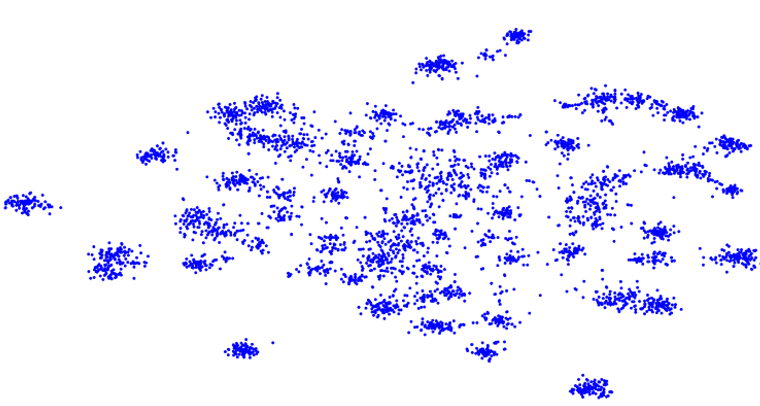
Built upon this main premise of features appearing clustered but shifted, local structure clustering (LSC) tries to to move the clusters and align them with the most likely class prediction. In particular, we would expect that nearest neighbors of target features share similar class labels with high probability. Based on this intuition, LSC encourages points close in feature space to have similar prediction to nearest neighbors, resulting in clusters moving jointly towards a common class.
In terms of implementation, LSC first buils a feature bank \mathcal{F}=\left\{f\left(\mathbf{x}_i\right)\right\}_{\mathbf{x}_i\in \mathcal{D}_t} (common approach in domain adaptation and unsupervised learning) and a score bank \mathcal{S}=\left\{p\left(\mathbf{x}_i\right)\right\}_{\mathbf{x}_i\in \mathcal{D}_t} with the predicted probabilities. The local structure clustering is achieved by encouraging consistent predictions between the m-nearest neighbors in feature space using the following loss \mathcal{L}_\text{LSC}=\underbrace{-\frac{1}{n_t}\sum_{i=1}^{n_t}\sum_{k\in \mathcal{N}_K^i} \log\left( \mathcal{S}_k^\intercal p\left(\mathbf{x}_i\right)\right)}_\text{Neighborhood consistency} + \underbrace{\sum_{c=1}^C \hat{p}_c \log \hat{p}_c}_\text{Diversity} where \mathcal{N}^i_{\left\{1,\ldots,K\right\}}=\left\{\mathcal{F}_j\vert \text{top-K}\left(\cos\left(f\left(\mathbf{x}_i\right),\mathcal{F}_j\right)\right),\forall\mathcal{F}_j\in\mathcal{F}\right\} is the K-nearest neighborhood of \mathbf{x}_i.
NRC: clustering using reciprocal neighbors (NeurIPS 2021)
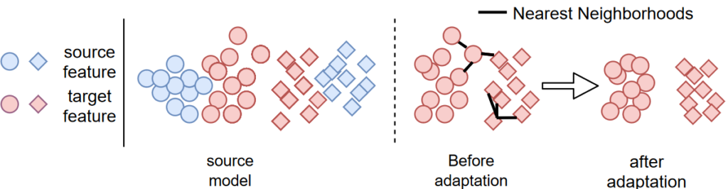
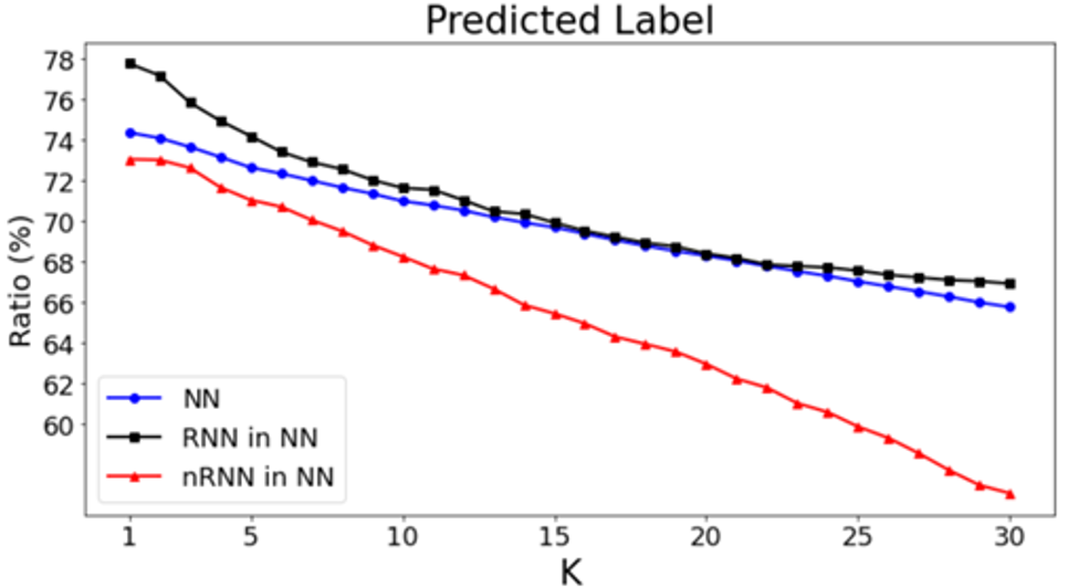
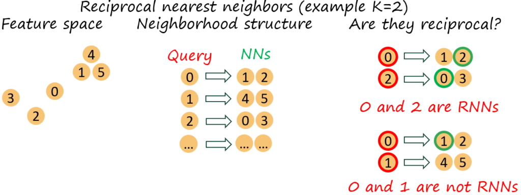
Neighborhood Reciprocity Clustering (NRC) is another clustering-based based on the same premise as LSC (i.e. target data under the source feature extractor appears clustered but shifted). In this case, there is also a second observation that motivates this method, consisting in the fact that reciprocal nearest neighbors (RNN) have the correct label with higher probability than non-reciprocal nearest neighbors (nRNN).
Now, first, what are reciprocal nearest neighbors? Simply put, a nearest neighbor of a point has this very point as nearest neighbor, i.e. i (with NNs \mathcal{N}_K^i) and j (with NNs \mathcal{N}_K^j) are reciprocal (K-)nearest neighbors if j \in \mathcal{N}_K^i \wedge i \in \mathcal{N}_M^j. The following figure illustrates the concept.
Another difference with previous works, is the use of expanded neighborhoods. We define the expanded neighborhood of point i as \mathcal{E}_M^i=\bigcup_{j\in \mathcal{N}_K^i}\mathcal{N}_M^j
Similar to LSC, NRC uses feature and score banks to find NNs and RNNs. Instead of implicitly assuming a binary affinity between pairs of samples (affinity 1 for neighbors, 0 for non-neighbors), NRC takes a more nuanced approach by defining an affinity matrix that assigns higher affinity (i.e. trust) to RNNs and lower to nRNNs. In particular, the affinity between K-NNs is defined as A_{i, j}=\begin{cases} 1 & \text{if }j \in\mathcal{N}_K^i \wedge i \in \mathcal{N}_M^j \\ r & \text{otherwise}, \end{cases}with r=0.1 in our experiments. Implicitly, the affinity between non-nearest neighbors is 0.
Once the affinity is determined, NRC computes the following loss \mathcal{L}_\text{NRC}=-\frac{1}{n_t}\sum_{i=1}^{n_t}\left[\underbrace{\sum_{k\in \mathcal{N}_K^i}A_{ik}\mathcal{S}_k^\intercal p\left(\mathbf{x}_i\right)}_\text{Class consistency}+\underbrace{\sum_{k\in \mathcal{N}_K^i}\sum_{m\in \mathcal{E}_M^k}r\mathcal{S}_m^\intercal p\left(\mathbf{x}_i\right)}_\text{Class consistency (expanded)}+\underbrace{\mathcal{S}_i^\intercal p\left(\mathbf{x}_i\right)}_\text{Self-regularization}\right]+ \lambda_\text{div}\underbrace{\sum_{c=1}^C \hat{p}_c \log \hat{p}_c}_\text{Diversity}
NRC++: taking care of outliers via reciprocal neighborhood density (TPAMI 2023)
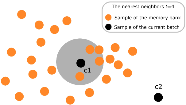
The performance of NRC may deteriorate in the presence of outliers in the current batch. NRC++ is an improved version of NRC that proposes to filter potential outliers prior to computing the loss. We can again leverage the relation between neighbors to estimate the neighborhood density, and use it as a means for outlier detection. In particular, for each feature \mathcal{F}_i in the feature bank we define the neighborhood density as \mathcal{O}_U^i=\left\{j\vert i\in \mathcal{N}_U^j\right\}. For example, in the following figure the point c1 lies in an area with high density, since it appears as U-NN of many other points. In contrast, c2 will rarely appear as U-NN of other points, suggesting that it is an outlier.
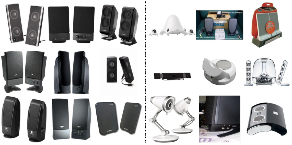
The following figure illustrates how neighboring features in high density areas correspond to similar images (inliers), while neighboring features in low density areas tend to include dissimilar images (potential outliers).
The final loss builds on top of that of NRC with an additional term corresponding to outlier detection \mathcal{L}_\text{NRC}=\mathcal{L}_\text{NRC}\underbrace{-\frac{1}{n_t}\sum_{i=1}^{n_t}\sum_{j\in \mathcal{O}_U^i}B_{ij}\mathcal{S}_j^\intercal p\left(\mathbf{x}_i\right)}_\text{Outlier removal} where the affinity is computed as B_{i, j}=\begin{cases} 1 & \text{if }j \in\mathcal{O}_U^i \cap \mathcal{N}_V^i \\ r & \text{otherwise}, \end{cases}
Method SF Office-31
(ResNet50)Office-Home
(ResNet50)VisDA
(ResNet101)PointDAN
(PointNet)Source model – 46.1 52.4 32.7 DANN ✗ – 57.6 57.4 44.2 MCD ✗ 86.5 64.1 – 45.3 PointDAN ✗ – – – 48.7 RSDA ✗ 91.1 70.9 75.8 – RWOT ✗ 90.8 – 84.0 – 3C-GAN ✓ 89.6 – 81.6 – SHOT ✓ 88.6 71.8 82.9 – BAIT ✓ 85.7 71.6 83.0 – HCL ✓ 89.8 – 83.5 – LSC ✓ – 71.3 85.4 – NRC ✓ 89.4 72.2 85.9 52.6 NRC++ ✓ 89.5 72.5 88.1 55.1
Generalized, continual and online SFUDA
Generalized SFUDA (ICCV 2021)
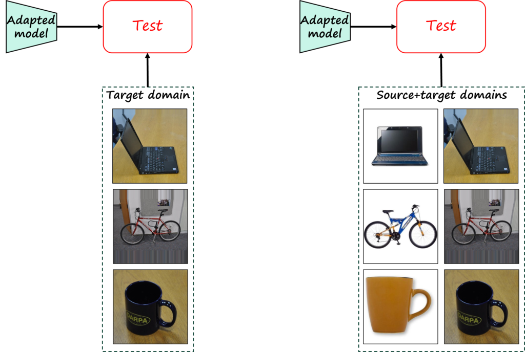
Together with LSC, we introduced a new setting, namely generalized SFUDA (GSFUDA). In contrast to SFUDA, where the domain adaptation method is evaluated only on the target domain, the GSFUDA setting requires evaluating the performance in both source and target domains.
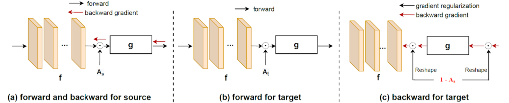
Thus, in order to address the GSFUDA setting we need to prevent catastrophic forgetting of the source domain. Inspired by works in continual learning (and in particular by HAT) that try to avoid exhausting all the model capacity in the current task, we propose to activate only some channels of the feature vector using sparse domain attention (SDA) masks \mathcal{A}_s and \mathcal{A}_t for source and target domains, respectively. Both masks are learned on the source domain and fixed during adaptation to target domain. The flow of information and gradient is illustrated in the following figure.
The following table shows an evaluation of LSC+SDA in the GSFUDA setting. Note that the performance in the target domain is slightly lower than in the SFUDA since we train with fewer source samples (80% for Office-Home, 90% for VisDA), leaving the remaining for test source performance.
| Method | Office-Home | VisDA | ||||
|---|---|---|---|---|---|---|
| S | T | H | S | T | H | |
| Source model | 99.6 | 48.1 | 64.9 | 83.9 | 59.2 | 68.6 |
| SHOT | 75.7 | 82.2 | 78.8 | 71.9 | 70.8 | 70.9 |
| LSC+SDA | 90.4 | 85.0 | 87.6 | 81.8 | 70.8 | 75.5 |
As expected, the model trained on source data has the best performance on the source domain, but poor performance on the target domain (which is precisely the motivation for domain adaptation). While SHOT is effective in greatly increasing the performance in the target domain, the performance in the source domain also drops significantly (i.e. catastrophic forgetting). LSC+SDA outperforms SHOT in the target domain while alleviating significantly the forgetting in the source domain, leading to a significantly higher harmonic mean that measures the combined performance.
Continual SFUDA (ICCV 2021)
Training first on source domain and then in a target domain, while evaluating on both is a special case of continual domain adaptation (note that the source-free constraint is implicit in continual learning, i.e. access to data of previous domains/tasks is not allowed). The extension to more than two domains is straightforward. The following table evaluates LSC+SDA for different permutations of four domains.
| Time | Train | Test | Train | Test | Train | Test | Train | Test | |||||||||||||||
|---|---|---|---|---|---|---|---|---|---|---|---|---|---|---|---|---|---|---|---|---|---|---|---|
| Ar | Cl | Pr | Rw | Cl | Ar | Pr | Rw | Pr | Ar | Cl | Rw | Rw | Ar | Cl | Pr | ||||||||
| t=1 | Ar | 74.5 | 42.0 | 61.3 | 68.2 | Cl | 82.2 | 49.7 | 60.0 | 61.2 | Pr | 92.0 | 49.7 | 41.0 | 71.0 | Rw | 86.0 | 63.0 | 45.7 | 77.6 | |||
| t=2 | Cl | 71.4 | 56.6 | 61.2 | 67.9 | Ar | 80.1 | 65.4 | 63.7 | 66.3 | Ar | 91.0 | 63.6 | 42.7 | 72.6 | Ar | 85.7 | 72.4 | 49.8 | 77.4 | |||
| t=3 | Pr | 70.9 | 55.7 | 73.0 | 71.2 | Pr | 79.7 | 63.2 | 72.9 | 68.2 | Cl | 89.2 | 61.8 | 53.1 | 70.4 | Cl | 80.7 | 68.9 | 59.1 | 73.4 | |||
| t=4 | Rw | 72.6 | 55.6 | 72.7 | 77.2 | Rw | 78.6 | 64.9 | 72.8 | 72.4 | Rw | 88.6 | 63.1 | 51.5 | 76.5 | Pr | 84.2 | 69.1 | 57.4 | 80.5 |
We can see that the performance in each domain increases after training with the corresponding domain data. After that point, the performance may degrade, but thanks to SDA, it drops only slightly. This behavior is consistent across the four domains and the four permutations.
Online SFUDA (CVIU 2023)
Together with BAIT, we also propose the online SFUDA setting, in which target data is only observed once (in contrast to offline SFUDA, where target data can be observed as many times as necessary). Note that the online setting is of high interests not only because of higher efficiency, but also because in many of such streaming scenarios storing target data locally may not be possible due to storage or privacy constraints.
The following table compares the performance of several methods in the offline and online settings. Note that BAIT is significantly better than SHOT in the online setting.
| Method | Source free | Offline | Online | ||||
|---|---|---|---|---|---|---|---|
| Office-31 | Office-Home | VisDA | Office-31 | Office-Home | VisDA | ||
| MCD | ✗ | – | – | 71.8 | 81.8 | 61.9 | 63.2 |
| MCD (w/o source) | ✓ | – | – | – | 79.5 | 59.2 | 59.2 |
| 3C-GAN | ✓ | 89.6 | – | 81.6 | – | – | – |
| SHOT | ✓ | 88.7 | 71.8 | 82.0 | 84.6 | 64.9 | 71.2 |
| BAIT | ✓ | 89.1 | 71.6 | 83.0 | 85.7 | 66.3 | 76.0 |
References
S. Yang, Y. Wang, J. van de Weijer, L. Herranz, S. Jui, “Generalized Source-free Domain Adaptation”, ICCV, 2021 [arxiv] [poster] [project].
Shiqi Yang, Y. Wang, J. van de Weijer, L. Herranz, S. Jui, “Exploiting the Intrinsic Neighborhood Structure for Source-free Domain Adaptation”, NeurIPS, 2021 [arxiv] [slides].
S. Yang, Y. Wang, J. van de Weijer, L. Herranz, S. Jui, “Casting a BAIT for Offline and Online Source-free Domain Adaptation”, Computer Vision and Image Unverstanding, 2023 (accepted) [arxiv].
S. Yang, Y. Wang, J. van de Weijer, L. Herranz, S. Jui, J. Yang, “ Trust your Good Friends: Source-free Domain Adaptation by Reciprocal Neighborhood Clustering”, IEEE Trans. on Pattern Analysis and Machine Intelligence, vol 45, no. 12, pp. 15883-15895, Dec. 2023 [arxiv][link].
J. Liang, D. Hu, J. Feng, “Do We Really Need to Access the Source Data? Source Hypothesis Transfer for Unsupervised Domain Adaptation”, ICML, 2020 [arxiv].
K. Saito, K. Watanabe, Y. Ushiku, T. Harada, “Maximum Classifier Discrepancy for Unsupervised Domain Adaptation”, CVPR, 2018 [arxiv].
Y. Fang, P.-T. Yap, W. Lin, H. Zhu, M. Liu, “Source-Free Unsupervised Domain Adaptation: A Survey”, arxiv 2023 [arxiv].
J. Serra, D. Suris, M. Miron, A. Karatzoglou, “Overcoming catastrophic forgetting with hard attention to the task”, ICML, 2018 [arxiv].