
Network compression and adaptation are generally considered as two independent problems, with compressed networks evaluated on the same dataset, and domain-adapted or task-adapted networks having the same architecture and size of the source networks. In our ICCV17 paper we show that considering adapting to the target domain or task jointly with compression can lead to significantly higher compression ratios. This intuitively makes sense, since if we are only interested in classifying birds, we can safely discard knowledge specifically related with classifying dogs, vehicles or plants. Let’s first introduce briefly these two fields.
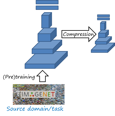
Network compression. A conventional deep neural network has several millions of parameters. These heavy networks lead to important hardware requirements such as large memory and high performance GPUs, yet still resulting in slow processing and high power consumption. This factors limits their deployment in constrained scenarios (e.g. mobile devices). Deep network compression addresses this problem by taking a heavy network and modifying the parameters to obtain a more compact, efficient and lightweight network while keeping a similar performance in the task. Other related approaches are network pruning and network distillation.
Transfer learning and adaptation. The parameters of a trained neural network (weights, in particular) capture the knowledge required to solve a particular task in a particular dataset. This knowledge can be transferred and re-purposed to better solve the same task in another domain (i.e. domain adaptation) or more generally to solve a different yet related task (i.e. transfer learning in general), by simply copying and adapting the weights. A typical case is using a large network, pretrained with a large classification dataset (e.g. ImageNet) to solve a source task (e.g. classify 1000 object categories) and then fine tune it with data from the narrower target domain (e.g. birds) to solve the target task (e.g. fine-grain classification of 200 types of birds). In this way the knowledge in the parameters of a powerful ImageNet classifier can be transferred and adapted to better solve the target task. Note that we may use the term domain in a broad sense where the task may also change.
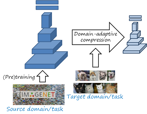
In contrast to conventional network compression, domain-adaptive network compression takes the data of the target domain and task into account during the compression process, being able to further reduce the size of the network by adapting to the target data.
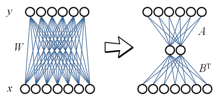
A commonly used method for compressing a layer of a neural network is (truncated) singular value decomposition (SVD). For example, considering a fully connected layer y = Wx + b, input x \in \mathbb{R}^n. output y \in \mathbb{R}^m and parametrized by the weight matrix W \in \mathbb{R}^{m\times n} and bias b \in \mathbb{R}^m, we can use SVD to factorize W as W = USV^T. An approximation can be obtained by truncating to the k most significant vectors as W \approx \hat W = \hat U\hat S\hat V^T, with \hat U \in \mathbb{R}^{m \times k}, \hat S \in \mathbb{R}^{k \times k}, \hat V \in \mathbb{R}^{n \times k}. This corresponds to decomposing the layer into two layers W=\left(\hat U\right)\left(\hat S\hat V^T\right)=B^T A. Note that the decomposition has fewer parameters when k is chosen such that nm > (n + m)k. The example below illustrates this idea, where n=7 and m=6. The original weight matrix contains 42 parameters, while the approximation with k=2 has 26 parameters in total).
Note that SVD is approximating a weight matrix that was designed to solve the source task in the source domain. However, in the case of different source and target domains this approximation is going to be less effective. Unfortunately, SVD has no information about the new target domain, so there is no way to adapt the approximation to the target domain.
Bias compensation
Rather than minimizing the approximation error of the weights ||W - \hat W||_F, as SVD does, we would be more interested in preserving similar outputs, that is, minimizing the representation error at the output ||Y - \hat Y||_F given X. Here the input matrix X \in \mathbb{R}^{n\times p} and output matrix Y \in \mathbb{R}^{m\times p} are obtained by concatenating the input and output representations of that layer for p samples of the target domain. Thus, we can represent the linear transformation of the whole set as
Y=WX + b1^T_p
where 1_p is a vector with ones of size p\times 1.
If we have already an approximated \hat W=B^T A, we can use these p samples from the target domain to slightly improve the approximation of the output feature Y by compensating the bias term
|| Y - \hat Y ||_F = || WX + b1_p^T - \left( \hat WX + \hat b1_p^T \right) ||_F= || \hat b1_p^T - \left( b1_p^T + \breve W X \right) ||_F
which is minimized by \hat b = b + \breve W X1_p = b + \breve W \bar x, where \bar x is the mean input to the layer. In this way, the information about the target domain is included through the bias term.
Domain adaptive low rank (DALR) matrix decomposition
SVD with bias compensation (SVD+BC) only considers target domain data for compensation but not during the decomposition. Besides, SVD does not enforce low rank in the decomposition, which is imposed later by truncating to k singular vectors. We further consider an explicit low rank decomposition W \approx \hat W = AB^T and directly optimize for A and B
\min_{A,B} || Y - \hat Y ||_F = \min_{A,B} || WX - AB^T X ||_F
where we assumed \hat b = b so we can remove them (we could compensate the bias later as shown before, although does not help much in this case). The resulting rank constrained regression problem can be written as
\begin{aligned}&\mathop {\arg \min }\limits_C & &|| Z - CX ||_F^2 + \lambda ||C||_F^2 \\ &\mathrm{s.t.} & &\mathrm{rank}(C) \le k \end{aligned}
where C=A B^T and Z=WX. Applying SVD on Z we obtain Z=USV^T. Then the matrices A and B are obtained as:
A = \hat U B = \hat U^T ZX^T \left( {XX^T + \lambda I} \right)^{-1}
where \hat U \in {R}^{m \times k} consists of the first k columns of U. This closed form solution is based on a method described here.
Results
The tables below show some representative results from our experiments, by comparing the accuracy for different compression rates of the fc6 layer of a VGG-19 network trained on ImageNet and then with target domains ImageNet (left table) and Caltech-UCSD Birds-200 (right table). SVD is able to keep the same accuracy with significantly fewer parameters. Bias compensation (SVC+BC) can further regain some additional accuracy points at very high compression rates, and DALR further allows for higher compression rates with still competitive accuracies. This difference is more significant when the source and target domains are different, since SVC+BC and DALR can adapt to the target domain.
| Dims kept | 32 | 64 | 128 | 256 | 512 | 1024 |
| Param (%) | 0.91 | 1.82 | 3.64 | 7.27 | 14.54 | 29.08 |
| SVD | 20.56 | 49.18 | 63.56 | 65.20 | 65.60 | 65.82 |
| SVD+BC | 26.59 | 53.46 | 63.79 | 54.18 | 65.67 | 65.78 |
| DALR | 33.57 | 55.50 | 63.94 | 65.37 | 65.72 | 65.80 |
| Dims kept | 32 | 64 | 128 | 256 | 512 | 1024 |
| Param (%) | 0.91 | 1.82 | 3.64 | 7.27 | 14.54 | 29.08 |
| SVD | 16.83 | 36.47 | 51.74 | 54.47 | 54.85 | 55.25 |
| SVD+BC | 27.91 | 46.00 | 53.50 | 54.83 | 55.21 | 55.44 |
| DALR | 48.81 | 54.51 | 55.78 | 55.85 | 55.71 | 55.82 |
In conclusion, domain-adaptive network compression can achieve higher compression rates when the target domain and task are taken into account during compression. We propose DALR, a simple method to implement this idea based on low rank decomposition. Our implementation in Tensorflow and Matconvnet is available here.