Yet another post about generative adversarial networks (GANs), pix2pix and CycleGAN. You can already find lots of webs with great introductions to GANs (such as here, here, here or here), pix2pix (here, with kittens, code and an interactive demo) and CycleGAN (here). Anyway, here are my two cents.
Generative modeling and sampling
One of the most fundamental problems in machine learning is estimating the true distribution given a collection of samples. If we effectively discover this true distribution wich a machine learning model, we could do many things, such as sampling from that distribution. Not surprisingly, this type of models are often known as generative models. Estimating a model is relatively easy in low dimensional spaces or if we have significant prior information about the structure of the probability distribution (e.g. thermal noise is known to follow Gaussian distributions, we just need to estimate the mean and variance). However, things get complicated for complex distributions in high dimensional spaces. That is the case in image generation.
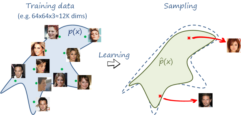
In the example above, we want to learn an approximation \hat p\left(x\right) of the true probability distribution p\left(x\right) of all the 64×64 color images that represent (realistic) faces (we have a dataset with a number of samples from p\left(x\right), i.e. real faces). If images are vectorized we have x\in \mathbb{R}^{12288}, since 64x64x3=12288. Even a small 64×64 image lies in a very high dimensional space of 12K dimensions. Now think of all the possible 64×64 images that represent faces and all the possible combinations of pixel values in 64×64 images. The former is just a tiny fraction of the latter, just like a needle in a haystack. And that is precisely our objective: to discover the tiny manifold embedded in a very high dimensional space where face images lie in. Current state-of-the-art generative models can generate realistic 1024×1024 images of faces (3M-dimensional space!!, check here). On a side remark: many of the generated faces look like real people, but they don’t exist in reality… disturbing, right?.
Another problem is that the distribution is very complex and we cannot assume a simple parametric model (e.g. a mixture of Gaussians). Together with high dimensionality, this makes it very difficult to be modeled directly with density estimation models. Only recently some new approaches have started to obtain good results. The most notable are variational autoencoders (VAE), autorregressive models (such as PixelCNN, PixelRNN) and generative adversarial networks (GANs). We will focus on the last one.
Generative adversarial networks (GANs)
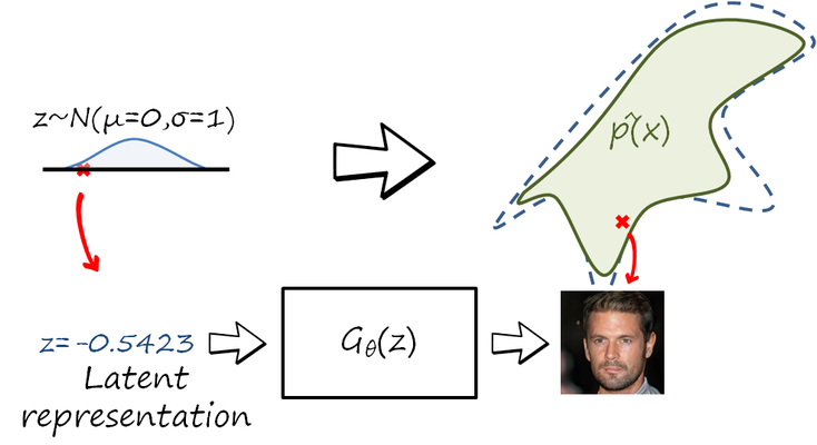
Instead of assuming a complex parametric model from which we generate new samples, many generative models use an indirect sampling approach. In this case, images are not sampled from the target high-dimensional space \hat p\left(x\right), but from a simple distribution (e.g. a normalized Gaussian) in a low-dimensional space known as latent space. Each latent vector z in this latent space is transformed into an image using a function G_\theta\left(z\right). With this indirect sampling mechanism the objective is now to learn the parameters \theta of the transformation, in such a way that the distribution of the transformed samples approximates p\left(x\right). As you can imagine, the family of transformations is implemented as a trainable neural network.
A possible way to solve that problem is learning a model that memorizes the training data in the parameters \theta and simply retrieves random training samples as output. In principle, that is something we want to avoid, because we are interested in p\left(x\right) rather than in the empirical distribution given by the training set. In other words, after training we would like to sample realistic yet unseen images.
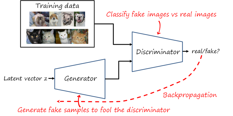
GANs are based on an adversarial setup where two networks, the generator G_{\theta_g}\left(z\right) and the discriminator D_{\theta_d}\left(x\right), compete to optimize their own objectives. The generator tries to generate images as realistic as possible. The discriminator tries to tell apart fake images coming from the generator and real images coming from the training set. Note that the generator never sees the training data directly. The game is formulated as the following minimax objective
\min_{\theta_g}\max_{\theta_d}\left[\mathbb{E}_{x\sim p_{data}\left(x \right)}\log D_{\theta_d}\left(x\right) + \mathbb{E}_{z\sim p\left(z \right)} \log \left(1 - D_{\theta_d}\left(G_{\theta_g}\left(z\right)\right)\right) \right ]
This can be addressed by alternatively optimizing the generator and the discriminator. The corresponding problem for the discriminator is
\max_{\theta_d}\left[\mathbb{E}_{x\sim p_{data}\left(x \right)}\log D_{\theta_d}\left(x\right) + \mathbb{E}_{z\sim p\left(z \right)} \log \left(1 - D_{\theta_d}\left(G_{\theta_g}\left(z\right)\right)\right) \right ]
and for the generator
\min_{\theta_g}\left[\mathbb{E}_{z\sim p\left(z \right)} \log \left(1 - D_{\theta_d}\left(G_{\theta_g}\left(z\right)\right)\right) \right ]
The authors (Goodfellow et al.) observed that optimizing this objective for the generator may lead to flat gradients (i.e. which carry very little information to update the generator and therefore learning will be difficult). They propose the following alternative that seems to provide more informative gradients and works better in practice
\max_{\theta_g}\left[\mathbb{E}_{z\sim p\left(z \right)} \log D_{\theta_d}\left(G_{\theta_g}\left(z\right)\right) \right ]
Optimizing this minimax problem is difficult and often unstable. However, many improvements have been proposed, including architectural improvements (e.g. DCGANs), better losses (e.g. Wasserstein distance), and better training strategies (e.g. PG-GANs). Current GANs are more stable to train and can generate images with larger resolutions.
Conditional GANs
So far so good, we can sample a random realistic image of a, say, animal. But we cannot control what kind of animal. Wouldn’t it be nice to tell the network the animal we want, e.g. a dog?
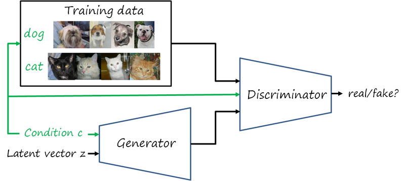
That is precisely the idea of conditional GANs, where an additional input is added to restrict the sampled images to those satisfying certain properties. For simplicity, we now focus on the semantic category c as condition (assuming that the training images are annotated with the corresponding category label). The task is now learning the joint distribution p_{data}\left(c,x\right) of labels and images, and then be able to sample from the conditional distribution p_{data}\left(x\vert c\right). This is achieved by modifying the original minimax objective to include the condition c in both the generator and discriminator (and also while sampling training/generated data)
\min_{\theta_g}\max_{\theta_d}\mathcal{L_\textnormal{cGAN}}\left( \theta_g,\theta_d\right )=\min_{\theta_g}\max_{\theta_d}\left[\mathbb{E}_{c,x \sim p_{data}\left(c,x\right)}\log D_{\theta_d}\left(c,x\right) + \mathbb{E}_{c\sim p_{data}\left(c\right),z\sim p_z\left(z \right)} \log \left(1 - D_{\theta_d}\left(c,G_{\theta_g}\left(c, z\right)\right)\right) \right ]
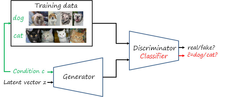
Another popular framework is Auxiliary Classifier GANs (AC-GANs), where in addition to the real/fake discrimination task, the discriminator network is augmented with an additional classification task: the generated imaged conditioned to a given category c should be classified as the same c.
Here we have considered categories as conditions. The power and flexibility of conditional GANs (or any other conditional image generation model) is that almost anything could be used as condition (in general we prefer conditions that can be represented as fixed-length vectors). Examples of problems that can be tackled with conditional GANs are image-to-image translation, text-to-image synthesis and attribute-to-image synthesis (where the conditions are image embeddings, text embeddings and attribute embeddings, respectively). We discuss the first one in the next sections.
Image-to-image translation
Most tasks in image processing and computer vision can be seen as transforming one input image into an output one (e.g. filtering, edge detection, image enhancement, colorization, restoration, denoising, semantic segmentation, depth extraction). The term image-to-image translation has been used recently to refer to general purpose methods that learn transformations directly from datasets with pairs of input and output images. These are some examples
For example, let us consider the problem of color to grayscale conversion. The solution to that problem is very simple, just average the RGB values of each pixel. Now let us consider the inverse problem of grayscale to color conversion (known as colorization). This is more complex, since there are many color values with the same grayscale value. In general, we need to figure out which of those colors are plausible, given the input grayscale image. But we need to resort to some high-level understanding of the image. For instance, if we understand the image is showing a face, then we can imagine the plausible skin colors that a particular face may have, obtained by our experience of having seen many faces during our life. Similarly, a colorization algorithm can learn to infer colors in grayscale faces after being trained with a dataset of color faces.
Another example is superresolution, which consists of upsampling a low resolution image to a realistic higher resolution one. Note that downsampling is trivial, by simply dropping high frequency information, but upsampling requires inferring those details. As in the previous example, the prior for these details can be learned from a suitable dataset.
These translations are not limited to photos, they could include other modalities and even translations between modalities (i.e. cross-modal translation). For example, semantic segmentation, where each RGB pixel is transformed to a semantic label. The inverse problem is photo image synthesis. As in the previous examples, the former is often a many-to-one problem (yet still challenging), while the latter is usually one-to-many (e.g. a region with the semantic label ‘car’ could have many RGB solutions, differing in color, texture, details, etc., yet all plausible).
Paired image-to-image translation
In many cases we can collect pairs of input-output images. For example, we can easily get edge images from color images (e.g. applying an edge detector), and use it to solve the more challenging problem of reconstructing photo images from edge images, as shown in the following figure
Now observe that we can consider the edge image as an input condition and then use a conditional GAN to generate the output image. This is the idea of pix2pix. The generator now is a bit more complicated, since it consists of an encoder followed by a decoder (implemented as a convolutional network followed by a deconvolutional network).
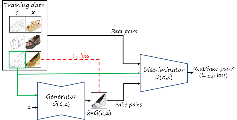
But that the optimization problem is exactly the same as in the category-conditional GAN described previously
\min_{\theta_g}\max_{\theta_d}\mathcal{L_\textnormal{cGAN}}\left( \theta_g,\theta_d\right )=\min_{\theta_g}\max_{\theta_d}\left[\mathbb{E}_{c,x\sim p_{data}\left(c,x\right)}\log D_{\theta_d}\left(c,x\right) + \mathbb{E}_{c\sim p_{data}\left(c\right),z\sim p_z\left(z \right)} \log \left(1 - D_{\theta_d}\left(c,G_{\theta_g}\left(z\right)\right)\right) \right ]
In addition to the conditional GAN loss, the authors also include a L_1 loss that forces the generated image for a given input to remain as similar as possible to the corresponding paired output ground truth image. This provides faster convergence and more stable training. This additional loss is
\mathcal{L_\textnormal{L1}}\left( \theta_g\right )=\mathbb{E}_{c,x \sim p_{data}\left(c,x \right ),z\sim p_z}\left \|x- G_{\theta_g}\left(c, z\right) \right \|_1
and the combined problem
\min_{\theta_g}\max_{\theta_d}\left[\mathcal{L_\textnormal{cGAN}}\left(\theta_g,\theta_d\right )+\lambda \mathcal{L_\textnormal{L1}}\left( \theta_g\right )\right]
Unpaired image-to-image translation
Now let us think of a more exotic translation, for example, horses to zebras. Given an image of a horse, can we get find the image of a zebra with the same background, same pose and aligned exactly with the original horse image? Probably not, so we cannot create an (input,output) pair, and therefore we cannot apply paired image-to-image translation.
However, if we relax the requirements and just collect a set of images with horses and a set of images with horses we can create a pair, but at the set level (in this case corresponding to two domains: horse and zebra).
In pix2pix we can generate an output image conditioned on the input one and compared with the corresponding output ground truth. In this case that is not possible. CycleGAN (and similar concurrent works, such as DiscoGAN and DualGAN) address this problem by learning at the same time the translation in both directions. Since images are generated in both domains, there are also two discriminators.
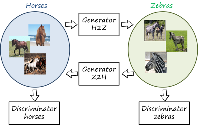
The main idea is to observe that transforming in one direction and then in the other back to the original domain (i.e. a cycle), ideally, the final image should be the same as the original. Therefore, we can compare both images and penalize when the difference is large (this is known as cycle consistency loss). Since we cannot compare with a reference output image, the reconstructed image is compared to the original input one (see figures below). The images generated are also evaluated by a discriminator for that particular domain.
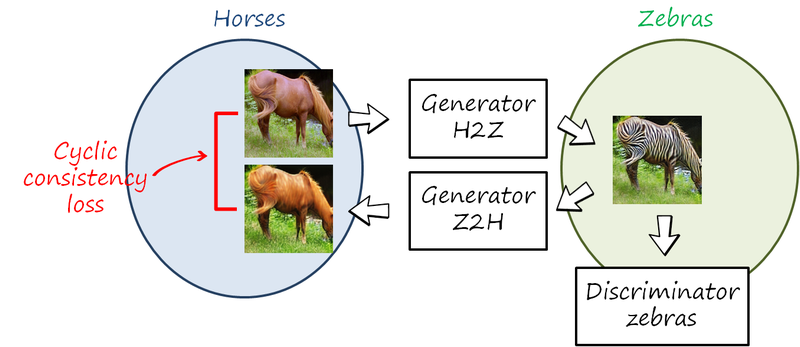
For convenience we refer to images x\in X from domain X (e.g. horses) and images x\in X from domain Y (e.g. zebras ). Let us illustrate the training process for the cycle horse-zebra-horse (X\rightarrow Y\rightarrow X). We also drop the random vector z used in previous cases. Now we have two translations y=G^\textnormal{XY}_{\theta_{xy}}\left(x\right) and x=G^\textnormal{YX}_{\theta_{yx}}\left(y\right) implemented using two generators G^\textnormal{XY}_{\theta_{xy}} and G^\textnormal{YX}_{\theta_{yx}}. The objective in this cycle is
\mathcal{L}^\textnormal{XY}_\textnormal{cGAN}\left( \theta_{xy},\theta_{yx},\theta_y\right )=\mathbb{E}_{y\sim p_{data}\left(y\right)}\log D^\textnormal{Y}_{\theta_y}\left(y\right) + \mathbb{E}_{x\sim p_{data}\left(x\right)}\log \left(1 - D^\textnormal{Y}_{\theta_y}\left(G^\textnormal{XY}_{\theta_g}\left(x\right)\right)\right)and the corresponding cycle consistency loss is
\mathcal{L}^\textnormal{XYX}_\textnormal{cyc}\left( \theta_{xy},\theta_{yx}\right )=\mathbb{E}_{x\sim p_{data}\left(x\right)}\left\| G^\textnormal{YX}_{\theta_{yx}}\left(G^\textnormal{XY}_{\theta_{xy}}\left(x\right)\right)-x \right\|_1 + \mathbb{E}_{y\sim p_{data}\left(y\right)}\left\| G^\textnormal{XY}_{\theta_{xy}}\left(G^\textnormal{YX}_{\theta_{yx}}\left(y\right)\right)-y \right\|_1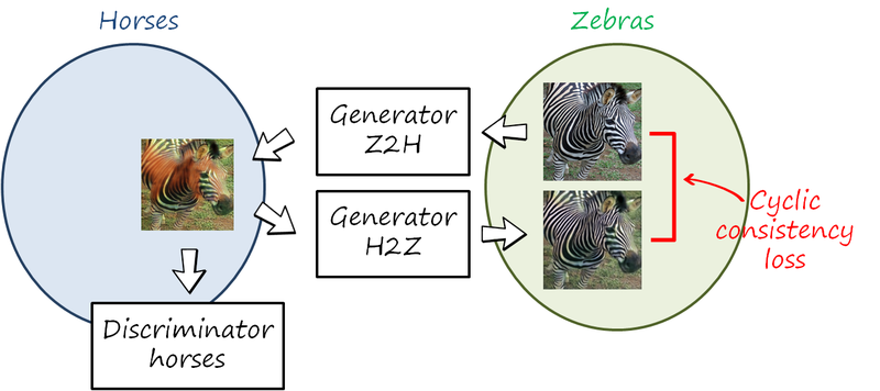
Similarly, the other cycle also has the corresponding losses \mathcal{L}^\textnormal{YX}_\textnormal{cGAN}\left( \theta_{xy},\theta_{yz},\theta_x\right ) and \mathcal{L}^\textnormal{YXY}_\textnormal{cyc}\left( \theta_{xy},\theta_{yx}\right). The full objective combines the four losses. And voila, here is your horse in zebra skin.